Shared Concepts · Hardware · 2026-09-18
How Collectives Move Data: Ring and Tree
Follow Ring and Tree implementations of the same All-Reduce result, and relate communication time to steps, data volume, and physical links.
Collective Communication: Combinations and Extensions described All-Reduce as combining matching array positions across GPUs and returning the result to everyone. That definition does not specify who sends to whom first.
A collective names the required result; its algorithm determines how transfers produce it. We will follow the same inputs through a Ring, which passes chunks between neighbors, and a Tree, which reduces and redistributes along branches. We will then compare steps and data volume, and distinguish the drawn connections from physical hardware.
Accumulating Chunks Around a Ring
A Ring assigns each participant a next peer, forming a cycle. Use four GPUs in the order 0 → 1 → 2 → 3 → 0. Each GPU can send to its next peer while receiving from its previous peer. They do not take turns with only one GPU working.
The goal is to sum matching input positions across four GPUs and give the resulting array to everyone. We will split this into two phases: first complete the sum for each chunk, then distribute the completed chunks to all GPUs. We do not need to build the entire sum on every GPU from the start.
Suppose each GPU holds a four-element array. Call the first position chunk A, the second B, the third C, and the fourth D. For example, the inputs for A on GPUs 0–3 are 1, 10, 100, and 1000, which sum to 1111. One element is one chunk here; a large array can instead be divided into chunks containing many elements.
Send each chunk to a neighbor, which adds its local input at the same position. Once the chunk has passed through the other three GPUs, all four contributions are included. Circulating different chunks simultaneously lets us leave one completed chunk on each GPU. This is Reduce-Scatter implemented with a ring.
The figure starts with the four GPUs’ inputs. Use Next to follow the three transfers in sequence. GPU positions and colors stay fixed. Each GPU keeps showing vector positions A, B, C, and D, with an outline around the position updated in this step. Arrows identify the chunk being sent.
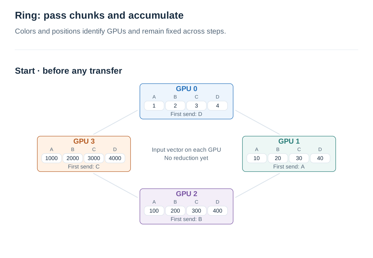
Starting stateView all steps together
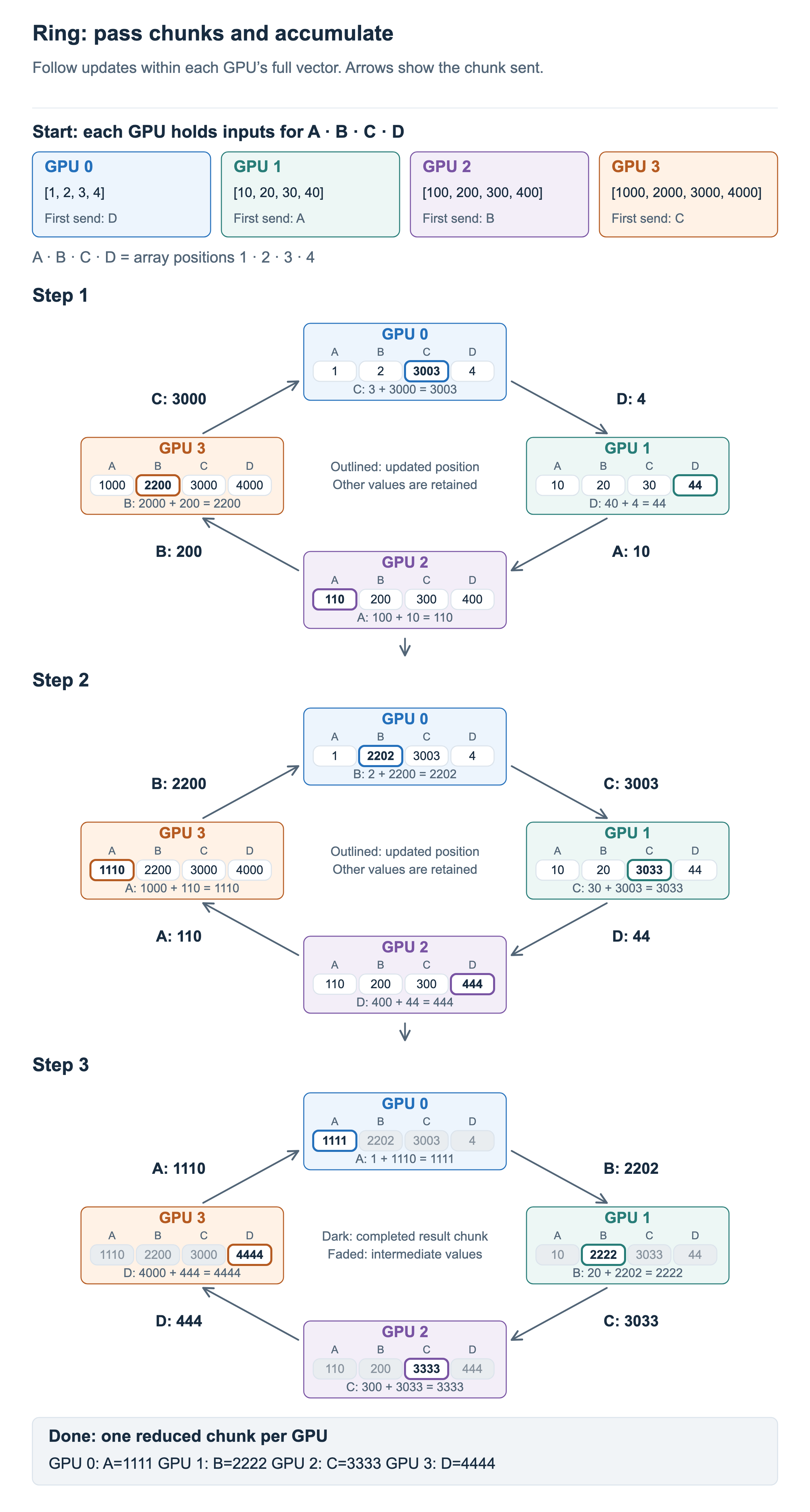
Use Next to follow the transfers. Click the figure to enlarge it.
Each GPU box shows the whole working vector. On receipt, the GPU adds the chunk to its local value at that position and keeps the other positions unchanged. On the first transfer, GPU 1 sends its A value, 10, to GPU 2. GPU 2 adds its local value 100 to obtain 110. GPU 3 then adds 1000 to obtain 1110. Finally, GPU 0 adds 1, completing A=1111.
Other chunks move simultaneously at other positions in the ring. After three transfers, GPUs 0, 1, 2, and 3 hold A=1111, B=2222, C=3333, and D=4444 respectively. In the final scene, each GPU’s dark cell is its completed result chunk. Faded cells contain values left during computation and are not part of the Reduce-Scatter output. No GPU has to collect the entire result first. The initial chunks were chosen to align final ownership with rank; library-internal chunk layouts can differ.
Distributing the Completed Chunks
Reduction is complete, but each GPU holds only part of the result. Forward these completed chunks in the same ring order. Retaining received chunks while forwarding them to the next neighbor gradually collects all chunks. This phase is All-Gather. The figure starts with only each GPU’s owned, completed result. Positions without a completed result are marked — and filled with received values in subsequent steps. These blanks do not mean memory was physically cleared; they mean the completed result for that position is not yet available.
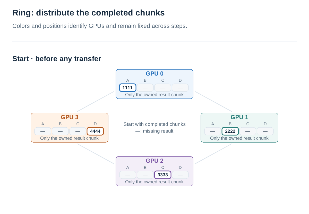
Starting stateView all steps together
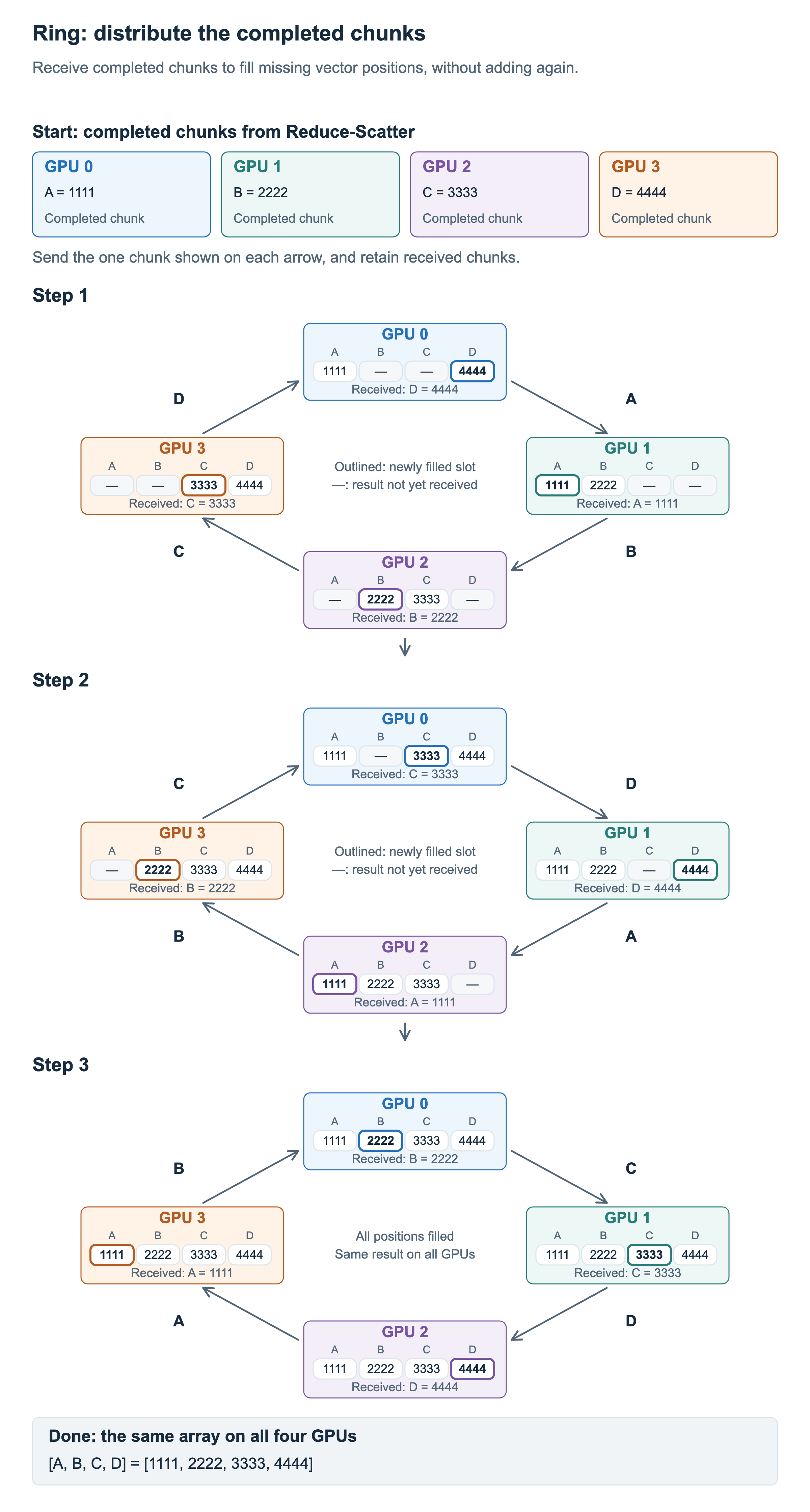
Use Next to follow the transfers. Click the figure to enlarge it.
On the first step, GPU 0 sends A to GPU 1 and receives D from GPU 3. It then forwards D while receiving C. After three steps, every GPU holds A through D. These are completed values, so they are copied without being added again.
An outline marks the newly filled position in each GPU’s vector. Each arrow identifies the one chunk sent in that step. A GPU does not send every chunk in its box: each GPU forwards one chunk per step. Three Reduce-Scatter steps plus three All-Gather steps complete the All-Reduce. These steps describe data dependencies; they do not require a separate CPU call or a global GPU barrier at every step.
Reducing and Broadcasting Through a Tree
A Tree defines parent–child relationships between participants. In a simple example, GPU 1 first sends to 0, and GPU 3 to 2. These two reductions proceed together, then GPU 2 sends its partial sum to GPU 0. Finally, the complete sum travels back along reversed edges. Use Next in the figure below to follow two reduction steps and two broadcast steps. GPU positions stay fixed. Dark arrows show the transfers performed in that step, and GPU boxes show values after the transfers.
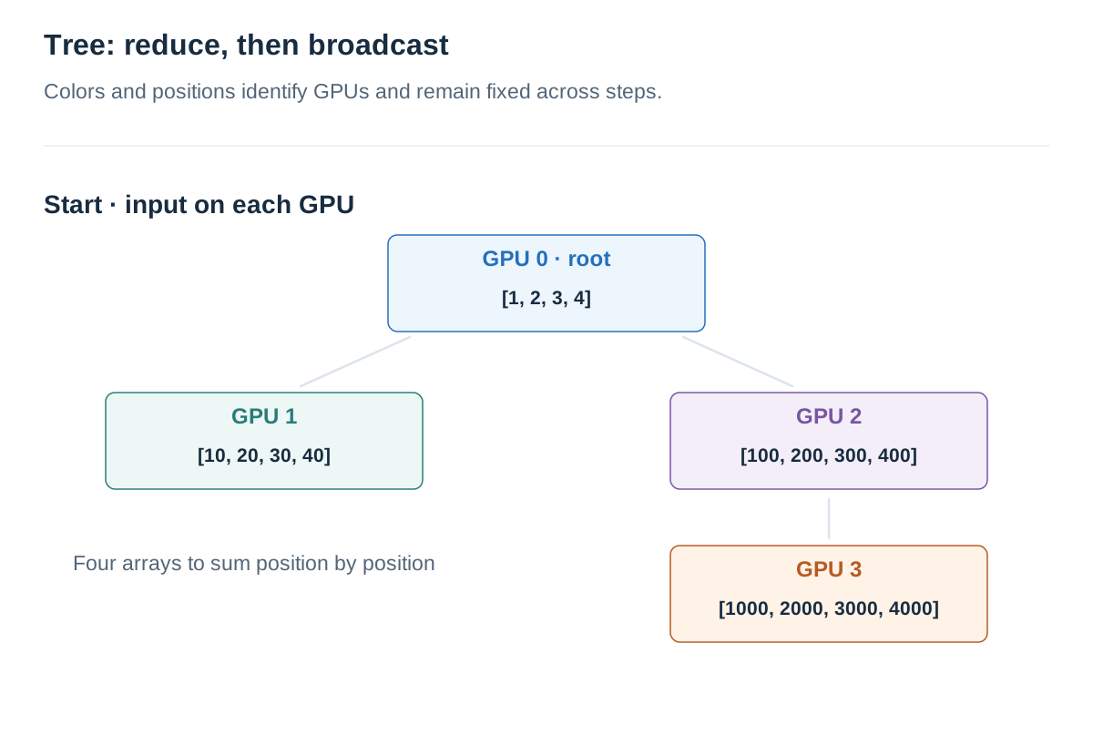
Starting stateView all steps together
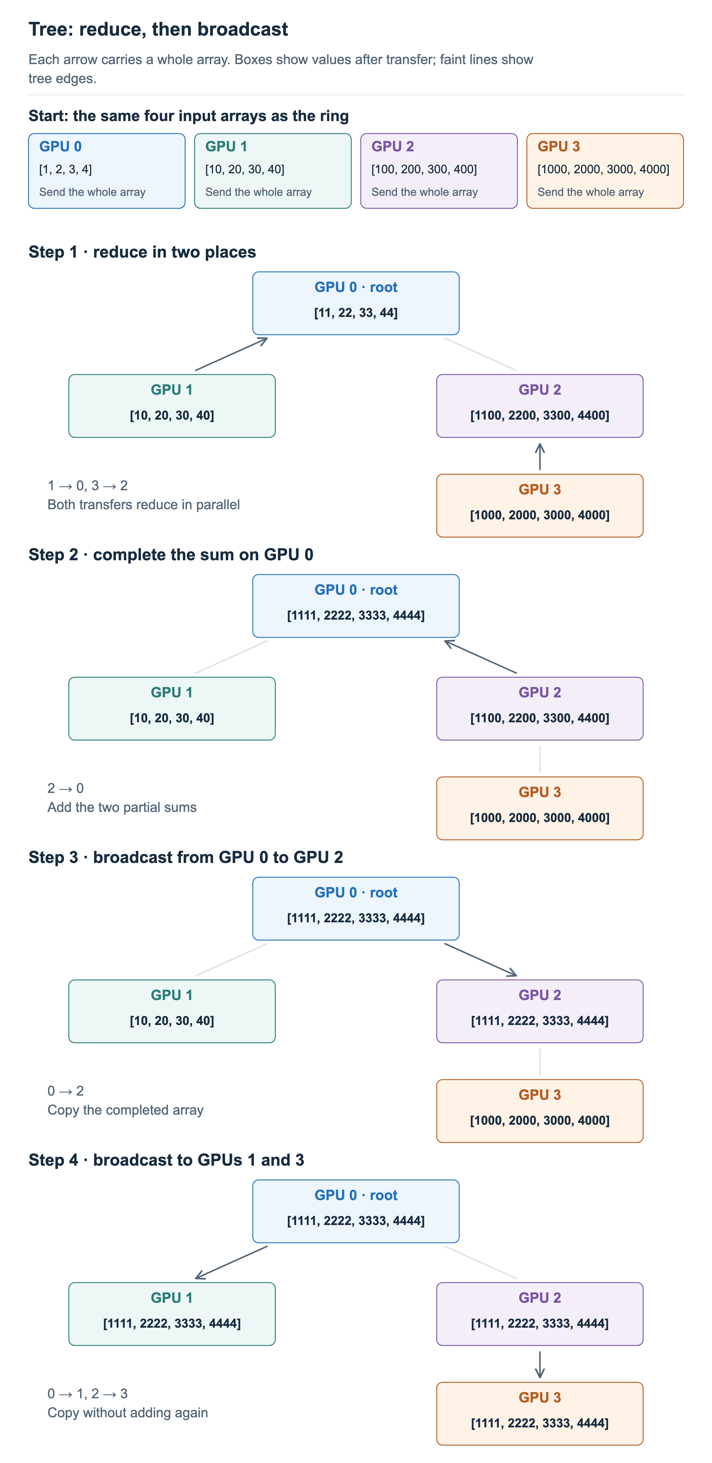
Use Next to follow the transfers. Click the figure to enlarge it.
Two reduction steps produce the full sum at GPU 0; two broadcast steps distribute it. There are fewer steps than in the ring example, but each transfer carries the entire array. Four steps therefore do not establish that this tree is faster than a six-step ring.
This is a simple teaching example. NCCL’s double binary tree explanation also describes splitting data between two trees to distribute internal-node load. Our simple tree does not reproduce the whole current NCCL Tree implementation.
Comparing Steps and Data Volume
Let p be the number of GPUs and M the input-array size per GPU in bytes. An evenly chunked Ring All-Reduce takes p−1 steps in each of its two phases. Each GPU sends M/p bytes per step:
Steps = 2(p − 1)
Total bytes sent per GPU = 2(p − 1)M/p
Received volume is the same, counted separately from the send volume above. With four GPUs, each sends 1.5 times the array size and receives the same amount. In the example tree, GPU 0 receives two arrays during reduction and sends two during broadcast; leaf GPU 1 sends and receives one each. Load differs between participants too.
When starting steps and waiting for dependent data are expensive, many steps can hurt. For large transfers, how evenly the available bandwidth is used matters more. Fewer steps and balanced traffic are different advantages to consider together. Real implementations can pipeline smaller pieces, so these counts should not be treated directly as an execution-time formula.
Distinguishing Logical Neighbors from Physical Links
A Ring does not require GPUs to be cabled in a circle. Transfers between logical neighbors can traverse switches or multiple physical links.
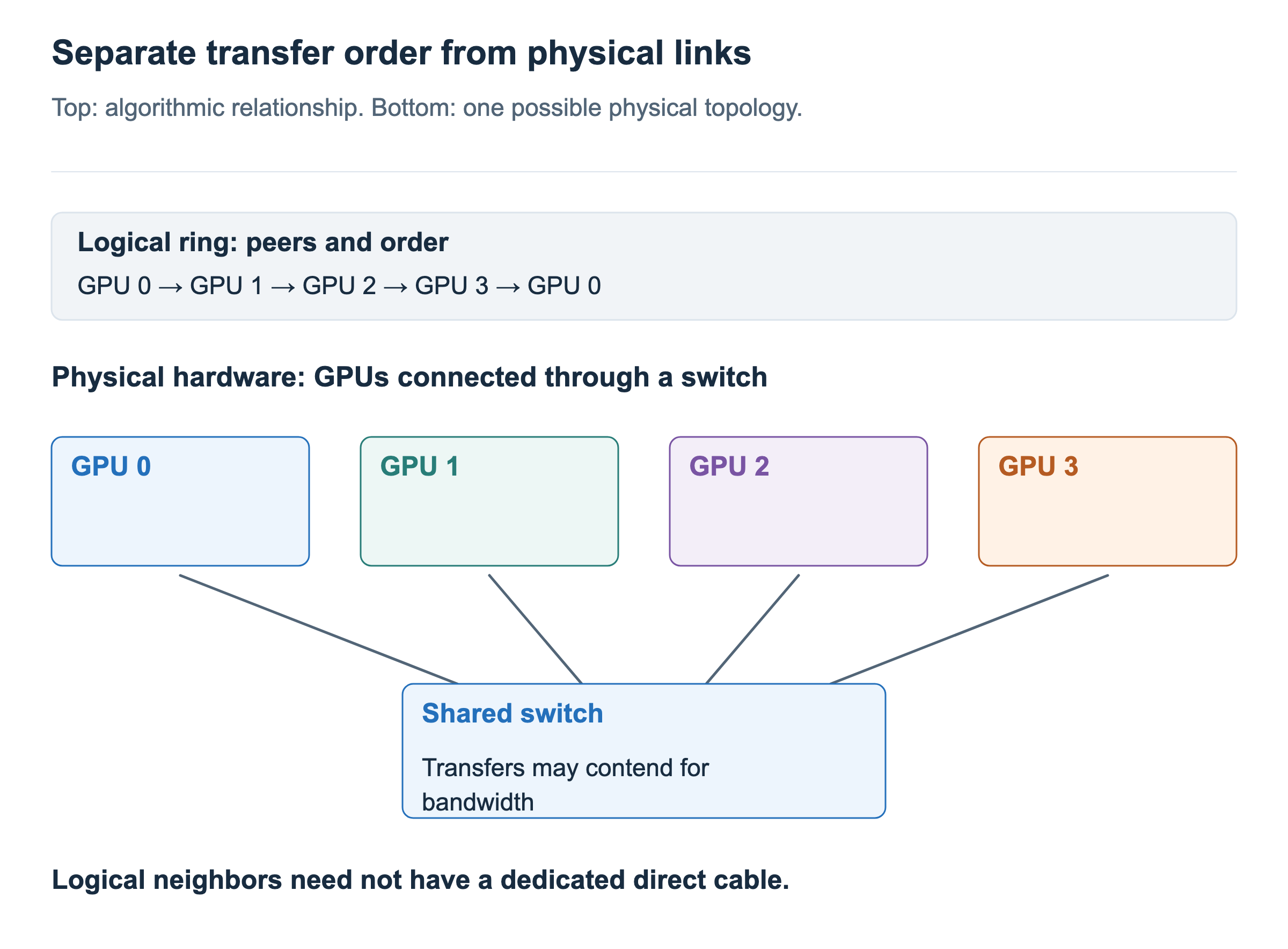
Transfers sharing a physical link compete for bandwidth. Changing the GPU order within the same ring can change the traffic crossing shared links. NVIDIA’s topology-aware collective explanation illustrates this relationship between physical connectivity and transfer order.
Developers normally request the collective and let the library select from available algorithms and paths. The current NCCL algorithm settings include choices beyond Ring and Tree. No algorithm should be presumed fastest for every message size and hardware configuration. Unlike our integer example, floating-point reductions can also differ in their last digits when addition order changes.
We can now distinguish the required result from its delivery method. Next, we will derive communication needs from how models and computation are placed.