Core Attention: Combining Information Across Tokens

In the previous article, we saw how the same input becomes Q, K and V, and how each vector’s components are grouped into multiple heads. The result of Core Attention passed through the output projection before being added to the residual stream. This article examines the internal computation of Core Attention that we left out before: computing scores between tokens with Q and K, turning those scores into weights, and taking a weighted sum of V.

Core Attention Computes Independently in Each Head

We will use the same MHA configuration as in the previous article. With T = 3 tokens, model dimension d = 8 and h = 2 heads, the dimension dh of one head is 4. Q, K and V each have shape 3 × 8. For each token, the first four components belong to Head 1 and the last four to Head 2. Figure 1 shows how these components are grouped by head and passed to Core Attention.

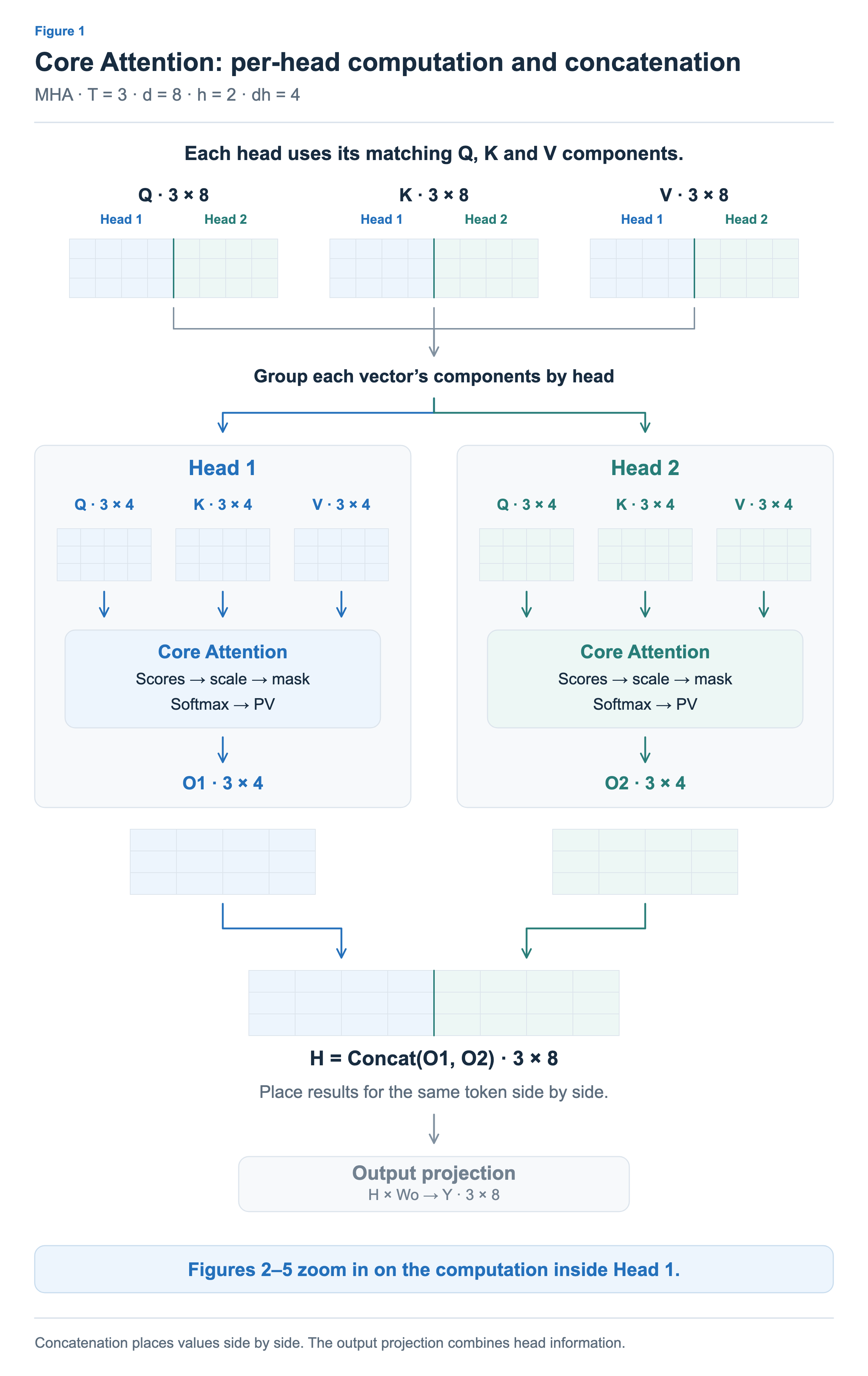
Q, K and V with the same head number participate in the computation together. Head 1 uses its own Q, K and V to produce O1, while Head 2 uses its own Q, K and V to produce O2. Each head computes results for all three tokens, but Q from one head is not multiplied by K from another. The computation follows the same steps, but the Q, K and V values differ, so the weights assigned to tokens and the results can differ as well.

O1 and O2 each have shape T × dh, or 3 × 4. Concatenating the results at the same token position (Concat) produces H with shape T × d, or 3 × 8. Concatenation places the values from each head side by side without changing them; the output projection then combines components from multiple heads. Figures 2–5 focus only on the computation inside Head 1. Head 2 independently follows the same steps using its own Q, K and V. The numerical values below are illustrative, not values taken from an actual model.

QKᵀ: Computing Scores Between Tokens

The first step is to pair each token in Q with each token in K and compute a score. Within one head, Q and K both have shape T × dh. Transposing K swaps its rows and columns, giving Kᵀ shape dh × T, so S = Q × Kᵀ has shape T × T. In this example, multiplying 3 × 4 by 4 × 3 produces a 3 × 3 score matrix S.

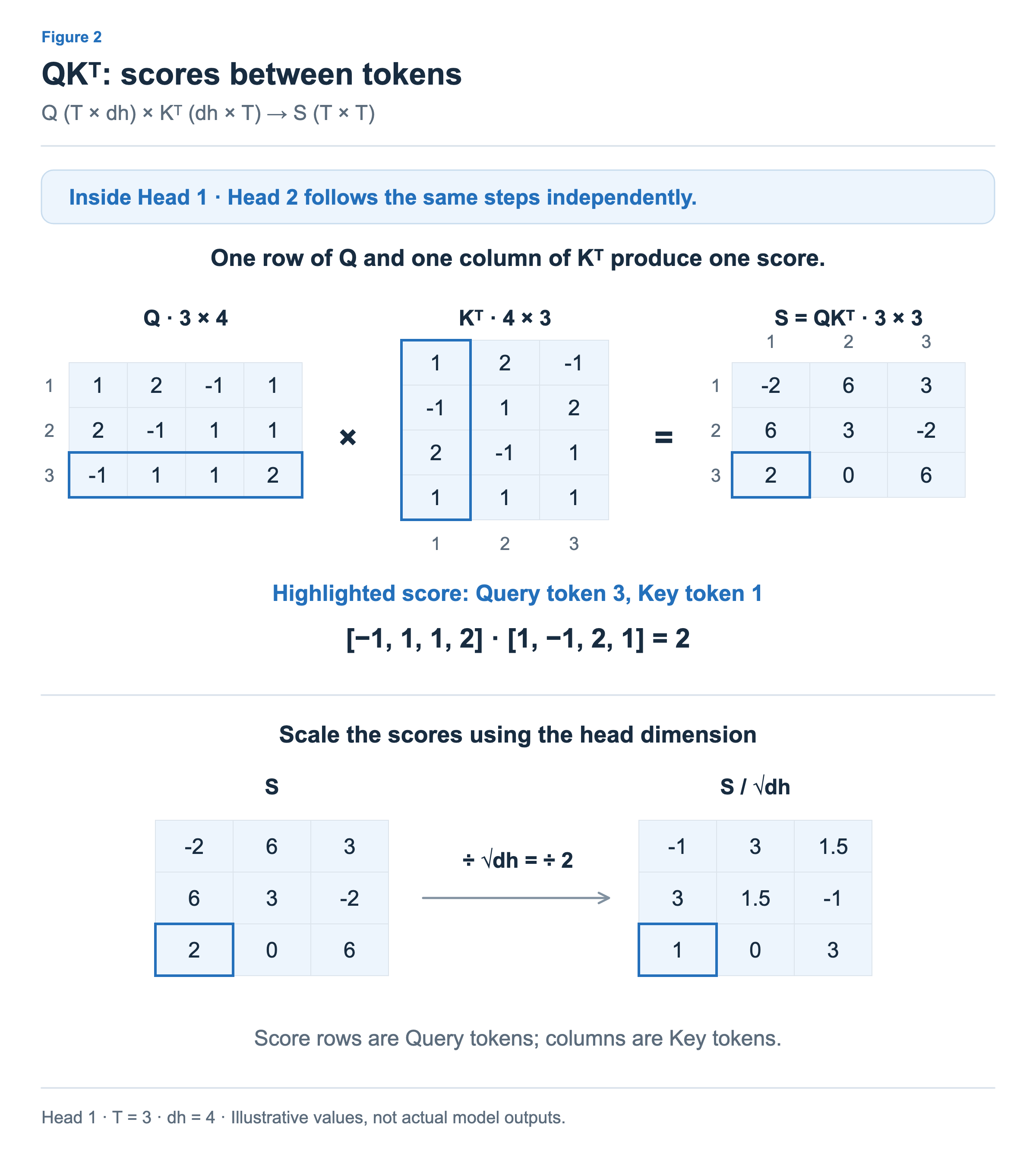
Each score is a dot product: multiply corresponding components of a Query vector and a Key vector, then add the products. In Figure 2, token 3’s Query is [−1, 1, 1, 2] and token 1’s Key is [1, −1, 2, 1]. Their score is therefore −1 × 1 + 1 × (−1) + 1 × 2 + 2 × 1 = 2. This value goes in the third row and first column of S. Rows correspond to Query tokens gathering information, and columns correspond to Key tokens being attended to. The third row of S, [2, 0, 6], compares token 3’s Query with the Keys of tokens 1, 2 and 3.

Next, we divide every value in S by √dh. A dot product adds the products of dh components, so its magnitude tends to grow as the dimension increases. If the score differences become too large, the Softmax that follows can concentrate the weights heavily on one token. Scaling adjusts their magnitude according to the head dimension. Here, dh = 4, so we divide all scores by 2. The highlighted score 2 becomes 1, and the third row [2, 0, 6] becomes [1, 0, 3].

Masking: Determining Which Tokens Can Be Attended To

So far, we have computed scores for each Query against every Key. In a decoder that predicts the next token, however, each position is restricted to attending to itself and earlier positions. When the output at a position is used to predict the next token, information from later tokens must not be available in advance. A causal mask defines this range of allowed positions.

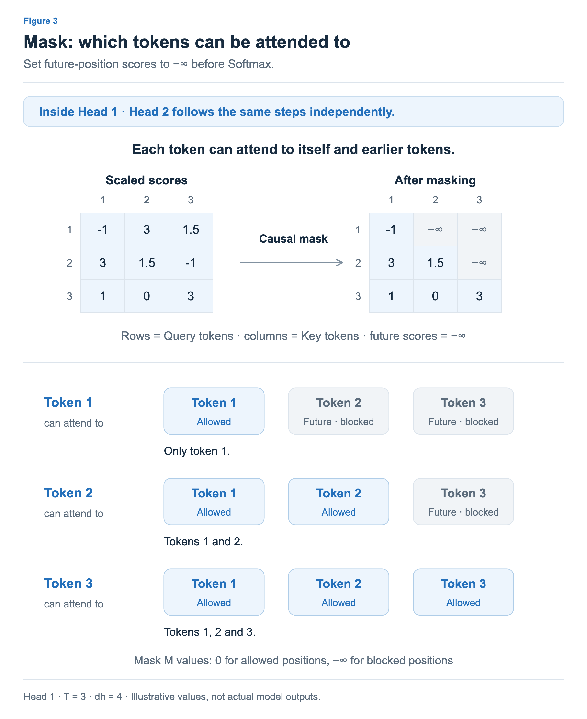
In Figure 3, token 1 attends only to token 1, token 2 to tokens 1 and 2, and token 3 to tokens 1, 2 and 3. In each row of the score matrix, the diagonal entry corresponds to the token itself, entries to its left to earlier tokens, and entries to its right to future tokens. We therefore set scores above the diagonal to −∞ and keep the rest. The second row [3, 1.5, −1] becomes [3, 1.5, −∞], while the third row [1, 0, 3] stays the same.

Mathematically, we can express this by adding a mask M to the scaled scores. M is a matrix with 0 at allowed positions and −∞ at excluded positions. Adding 0 leaves a score unchanged, while adding −∞ makes it −∞. “Mask M values” in the figure refers to these added values.

Softmax: Turning Scores Into Weights

We will now turn the scores between tokens into weights to multiply each Value by. Softmax converts the scores in a row into nonnegative weights that sum to 1. The computation is P = softmax(S / √dh + M), applied within one row corresponding to a single Query token. Each entry in P indicates how much to incorporate the Value of the token in that column.

Softmax applies the exponential function exp to each score, then divides by the sum of the resulting values in that row. For token 3 in Figure 4, the scores are [1, 0, 3]. Converting them to [e¹, e⁰, e³] and dividing by e¹ + e⁰ + e³ gives weights of approximately [0.114, 0.042, 0.844]. Within the same row, a higher score receives a larger weight. In this example, token 3 assigns the largest weight to its own Value, while also incorporating the Values of tokens 1 and 2.

Applying the exponential function to the masked score −∞ gives 0, so that position’s weight is also 0. Token 1 has only one allowed position, giving [1, 0, 0], while token 2 receives approximately [0.818, 0.182, 0]. A token with score 0 also participates in the weighted sum. The second score in token 3’s row is 0, but e⁰ = 1, so it receives a weight of approximately 0.042. P is displayed rounded to three decimal places in the figure.

PV: Taking a Weighted Sum of Value Vectors

Finally, we combine the Value vectors using the weights in P. The computation is O = P × V. P has shape T × T and V has shape T × dh, so O has shape T × dh. In this example, multiplying 3 × 3 by 3 × 4 produces a 3 × 4 output. One row of P contains the weights for one Query token, and each row of V is the corresponding token’s Value vector.

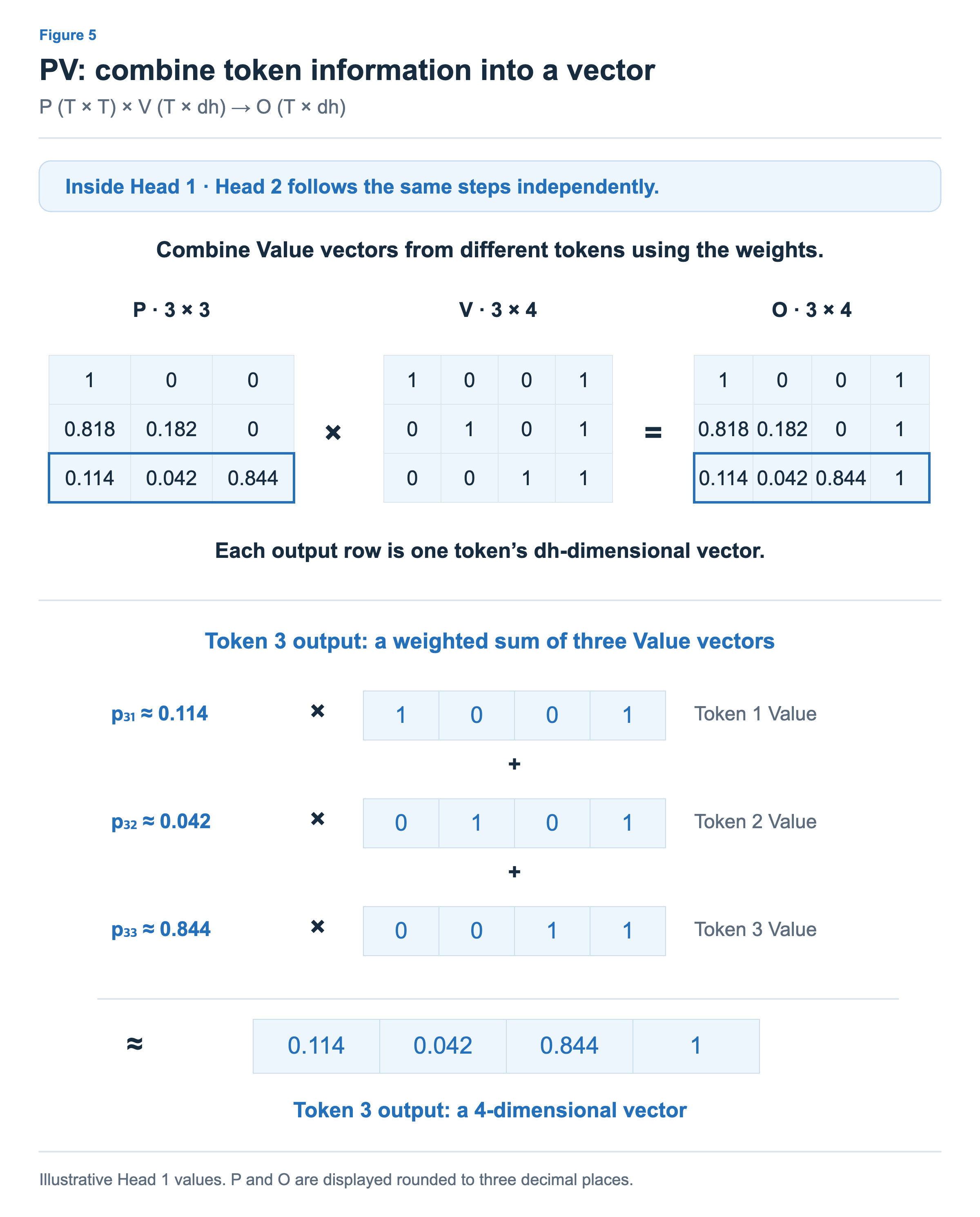
In Figure 5, token 3’s output can be read as token 1’s Value × 0.114 + token 2’s Value × 0.042 + token 3’s Value × 0.844. Each weight multiplies all four components of its corresponding Value vector. Adding the three results component by component gives approximately [0.114, 0.042, 0.844, 1]. The last component is 1 because all three Values have a last component of 1, and the weights sum to 1.

The other tokens follow the same process. Token 1 has weights [1, 0, 0], so its own Value passes through as its output. Token 2 takes a weighted sum of the Values of tokens 1 and 2, while token 3 takes a weighted sum of all three. Combining information from multiple tokens preserves the output vector’s dimension dh. Each token produces four components in this example, so Head 1’s full output O has the same 3 × 4 shape as input V.

Core Attention computes scores between tokens with Q and K, uses a mask to define which positions can be attended to, and gathers V according to the weights produced by Softmax. Q and K determine which tokens to incorporate and how much, while V provides the information being combined. Returning to the full flow in Figure 1, the results computed in each head are concatenated at matching token positions and passed to the output projection.