Inference Metrics: Latency and Throughput

Earlier articles examined how requests are batched and executed, how KV cache is managed, and how some requests can be paused and resumed when space runs out. We now need criteria for judging how well that process works. One request finishing quickly does not mean that the server processed many requests, and completing many requests does not mean that every user waited briefly.

This article first breaks down the waits experienced by one user, then considers how much work the server handles over a period of time. We will then examine output gaps and differences in request latency that averages can hide, before connecting them to goodput: work completed within latency targets. The figures use illustrative values to explain the principles, not measured performance results.

Latency within one request

Consider a user sending a request and receiving an answer. Initially, the user waits with no output. After the first token arrives, further tokens arrive in sequence, and eventually the request ends. Even within one request, the wait for the first answer can be distinguished from the intervals at which the answer continues.

Here we will use the times at which the client submits the request and receives output. For clarity, assume that each output chunk contains one token. In Figure 1, the client submits a request at 0ms, receives tokens at 100ms, 130ms, and 170ms, and observes the request ending at 180ms.

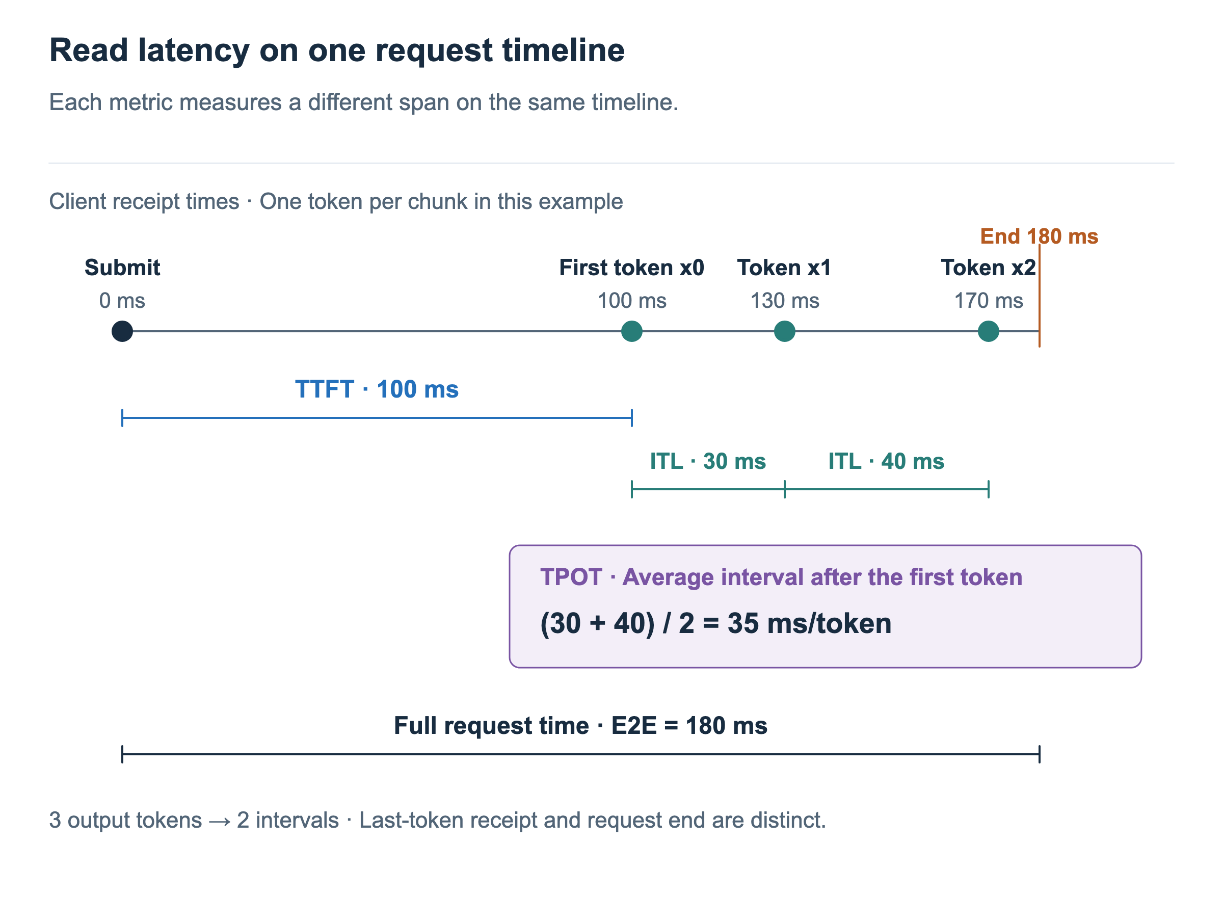
The request is submitted at 0ms, tokens x0, x1, and x2 arrive at 100, 130, and 170ms, and the request ends at 180ms. TTFT is 100ms, ITLs are 30 and 40ms, TPOT is 35ms/token, and total request time is 180ms. — Figure 1. Different starting and ending points on the same request produce different latency metrics.

TTFT (Time to First Token) is the time from submitting the request to receiving the first output token. In the figure, it is 100 − 0 = 100ms. Since this measures the user’s wait for the first answer, it can include queueing, input processing, and output delivery. The entire TTFT should therefore not be interpreted as prefill computation time.

ITL (Inter-Token Latency) is the interval between consecutive output tokens. From x0 to x1, it is 130 − 100 = 30ms; from x1 to x2, it is 170 − 130 = 40ms. A request has multiple such values, each revealing how long the user waited during a particular part of generation.

TPOT (Time per Output Token) will be defined here as the per-request average of the output intervals after the first token. With 3 output tokens, there are 2 intervals, so the figure’s TPOT is (30 + 40) / 2 = 35ms/token. More generally, for N output tokens:

TPOT = (Last-token receipt time − First-token receipt time) / (N − 1)

The wait for the first token is excluded from this average. If only one token is received, there is no interval between tokens, so TPOT cannot be calculated under this definition. Treating such a request as 0ms could distort the average; it needs separate handling.

Total request time (E2E latency) is the time from submitting the request to observing its end. In the figure, this is 180ms. The last token arrived at 170ms, but the end was observed at 180ms, so those endpoints differ. A tool’s result can vary depending on whether it measures through the last token or through the end. In particular, if a tool uses total request time to calculate TPOT, check that time’s endpoint as well.

These definitions measure latency as observed by the user. After the model selects a token, text conversion, output chunk assembly, and transmission still follow, so internal generation times and receipt times can differ. If a chunk contains multiple tokens, chunk arrival intervals alone also cannot reveal individual token intervals. Distinguish internal execution timing from client receipt timing, and state the boundaries used.

Throughput across requests

Having measured one request’s latency, let us widen the view to the whole server. The server handles multiple requests together. Even if each request receives output at a steady pace, the total amount of output varies with the number of requests progressing concurrently.

Throughput is the amount of work handled over a period of time. Counting completed requests gives request throughput; counting output tokens gives output token throughput. Their counting units differ, so they should be labeled separately.

Figure 2 shows a 10-second observation window separate from the earlier 180ms example. Requests A, B, and C all start and complete within this window. Open circles mark submission, filled dots mark output token receipt, and check marks indicate completion.

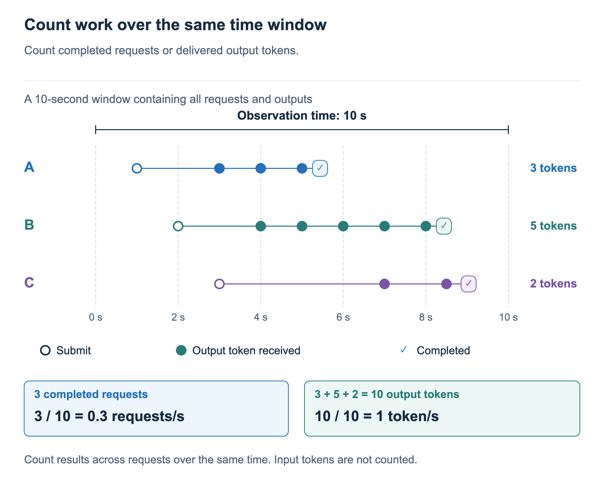
Requests A, B, and C overlap and all complete within a 10-second observation window. They produce 3, 5, and 2 output tokens. Counting 3 completed requests gives 0.3 requests/s; counting 10 output tokens gives 1 token/s. — Figure 2. Divide completed requests and output tokens across requests by the same observation time.

There are 3 check marks, meaning 3 completed requests. Request throughput is therefore 3 / 10 = 0.3 requests/s. There are 3 output dots for A, 5 for B, and 2 for C, totaling 10, so output token throughput is 10 / 10 = 1 token/s. The execution is the same, but changing what goes into the numerator produces a different metric.

The generation rate obtained by taking the inverse of one request’s TPOT is not this server-wide throughput. Other requests also produce output during the same time, as the figure shows. We have also counted only output tokens here. If a reported token throughput combines input and output, that should be stated.

This example places every request and output inside the observation window. Real measurements can include requests that arrived before the window began or remain active after it ends. Along with deciding whether to count completed requests or output tokens received within the window, define where the observation time starts and ends.

Output gaps hidden by an average

So far, we have distinguished how long one request waited from how much work the server handled. Now let us examine what can be missed when results are summarized by a single average. First, return to the output intervals within one request.

A TPOT of 35ms/token does not mean that output always arrives every 35ms. In Figure 3, both cases take 70ms from the first token to the last. The upper case has two waits of 35ms, while the lower case has a 5ms wait followed by a 65ms wait.

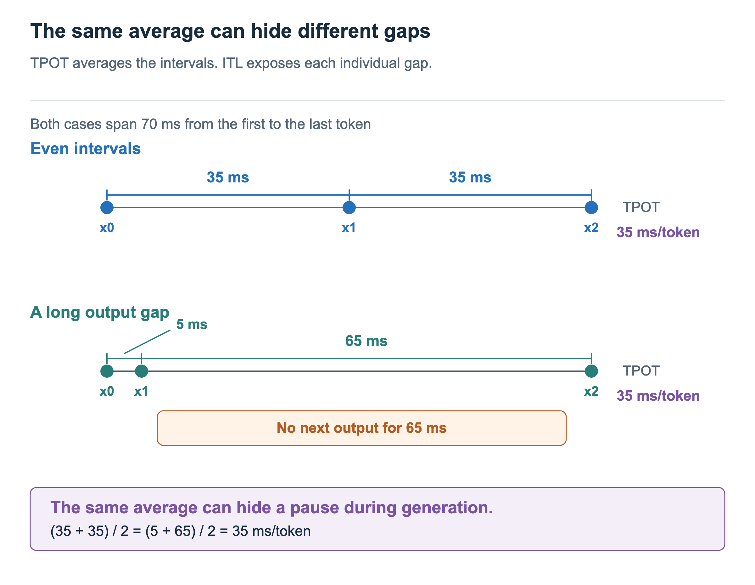
Two output streams span 70ms between their first and last tokens. The upper intervals are 35 and 35ms; the lower intervals are 5 and 65ms. Both have TPOT 35ms/token, but the lower stream has a 65ms gap without new output. — Figure 3. Even with the same TPOT, individual token intervals can reveal a long pause during generation.

In both cases, the intervals sum to 70ms and there are 2 of them, so TPOT is identical. In the lower case, however, the user receives x1 and then experiences a long period without further output. The same average generation rate does not establish that output arrived steadily.

Recall the preemption example: a paused request produced no new output while waiting to resume and rebuilding its KV. Averaging such a long interval together with shorter ones can make its impact look smaller. Examining actual ITLs alongside per-request TPOT reveals pauses that the average alone does not show.

Request latency distributions and percentiles

Next, consider differences across requests. Most requests may receive their first token quickly while some wait much longer. The average TTFT across all requests does not tell us how long those users waited.

Figure 4 sorts the TTFTs of 20 requests from shortest to longest. Each bar represents one request, and its height shows the wait for the first token. A few requests on the right have much longer latency than the others. The long end of such a distribution is called the tail, and latency in that region is called tail latency.

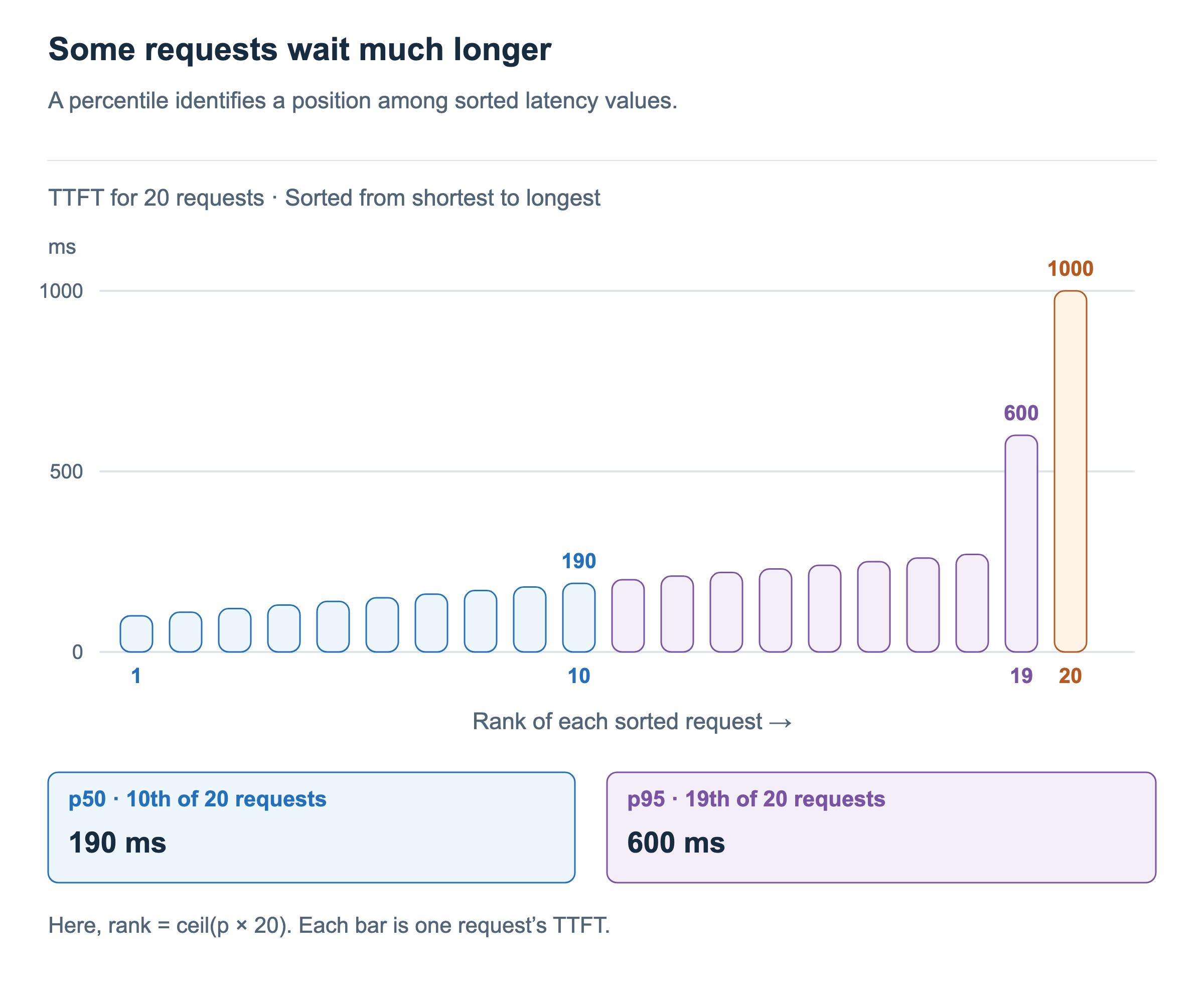
TTFT bars for 20 requests sorted from shortest to longest. The 10th value is 190ms, the 19th is 600ms, and the last is 1000ms. With a rank-rounding-up rule, p50 is 190ms and p95 is 600ms. — Figure 4. Sorting request latencies distinguishes the majority of requests from those that waited longer.

A percentile examines the position corresponding to a particular proportion of these sorted values. p50 examines the 50% point, and p95 the 95% point. For this example, we will use rank = ceil(proportion × number of requests), substituting 0.50 for p50 and 0.95 for p95.

With 20 requests, p50 is the 10th value, 190ms, and p95 is the 19th value, 600ms. In this example, 10 requests have TTFT at or below 190ms, and 19 have TTFT at or below 600ms. The remaining request waits 1000ms. A p95 of 600ms therefore does not mean that every request received its first token within 600ms.

Some percentile methods interpolate between values. Even with the same samples, the result can vary with the tool’s calculation rule, so comparisons should use the same rule. The 20 samples in the figure illustrate the principle; estimating an extreme tail such as p99 in practice requires enough samples.

What goes into the distribution matters too. A distribution of per-request TTFTs, a distribution of per-request average TPOTs, and a distribution of all token intervals are different. In particular, pooling all ITLs gives more samples to requests with longer outputs. Do not compare the label “p99” alone: check which metric and which samples were sorted.

Throughput that meets latency targets

We can now consider latency and throughput together. A server may complete many requests, yet still fall short of the user’s expectations if the first answer arrives too late or generation is too slow. Setting the latency targets a service needs lets us count how many completed requests met them.

Figure 5 sets two conditions for each request: TTFT at or below 1 second and TPOT at or below 50ms/token. These are illustrative targets, not criteria suited to every service. A request counts as passing only if it satisfies both conditions.

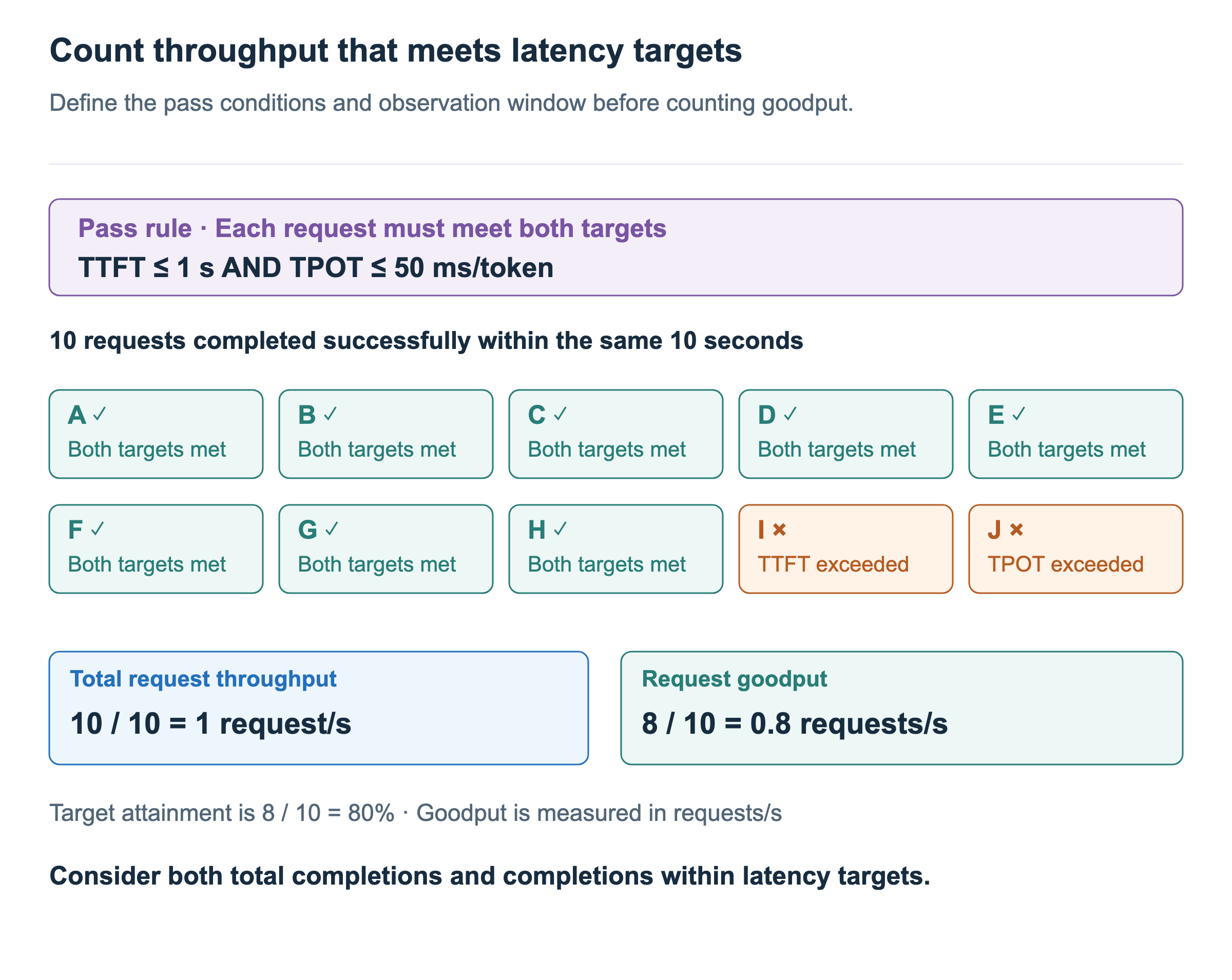
Of 10 requests completed successfully within 10 seconds, requests A through H meet both TTFT at or below 1 second and TPOT at or below 50ms/token. I exceeds the TTFT target and J the TPOT target. Total throughput is 1 request/s, goodput is 0.8 requests/s, and target attainment is 80%. — Figure 5. Calculate goodput by counting only completed requests that meet every latency target.

Ten requests completed successfully during the 10-second observation window, so total request throughput is 10 / 10 = 1 request/s. Only 8, however, met both targets. The remaining 2 also completed, but one was late with its first response and the other exceeded the target for average output interval.

Here, request goodput is the number of successfully completed requests that meet all latency targets, divided by observation time. In the figure, it is 8 / 10 = 0.8 requests/s. The Inference Perf goodput documentation also describes counting requests that both complete successfully and satisfy the specified conditions.

Target attainment is a separate value. In this example, the fraction of completed requests that met the targets is 8 / 10 = 80%. The denominator for attainment is a request count, whereas the denominator for goodput is time. Looking at total throughput, target attainment, and goodput together distinguishes how much work completed from how much met the targets.

The pass conditions must also accompany the result. Here we used TTFT and per-request average TPOT. As we saw earlier, even a TPOT within the target can leave a single long output gap. Placing an upper bound on every token interval is a different condition from the one in this figure. The name “goodput” alone does not tell us which aspects of the user experience were satisfied.

Compare optimizations under the same conditions

Comparing optimizations with these metrics also requires matching the requests and load. Short and long inputs have different prefill costs, while changing output length changes the number of decode iterations and how long KV is retained. Even for the same model, sparse requests and bursts of requests produce different waits.

At a minimum, record input and output lengths, request arrival rate and concurrency limits, the model and hardware, and the measurement window. Arrival rate is the number of new requests per second; concurrency is the number of requests not yet finished. A test that maintains a fixed number of requests, sending another whenever one completes, can reduce its actual arrival rate as responses slow down. It cannot be treated as the same load as a test that continues sending requests at a fixed rate.

Record how rejected, failed, and canceled requests were handled as well as successfully completed ones. This distinguishes raising the target-attainment fraction by admitting fewer requests from increasing the actual throughput that meets targets under the same offered load.

When examining later optimizations, we can now ask which waits were reduced, how overall throughput changed, whether long delays remain for some requests, and whether throughput within the specified targets increased. The later discussions of scheduling and admission control will build on these criteria to explain how resources are allocated to requests.