Shared Concepts · Hardware · 2026-09-18
PP: Partition and Execute Model Layers
Place model layers across GPUs, then split the same batch into microbatches to overlap computation for different inputs.
So far, we have partitioned features or tokens within a layer. A model also has an ordering in which one layer uses the preceding layer’s output. Pipeline parallelism (PP) places these layers across multiple GPUs. Each GPU holds part of the model, allowing a model that is difficult to fit on one GPU to be distributed across several.
Partitioning layers does not immediately make every GPU compute at once. Later GPUs must wait for results from earlier GPUs. This article first examines layer placement and the directions of forward and backward passes. We then examine how much GPUs wait when a whole batch is passed onward. To reduce that waiting, we split the batch into smaller groups and compare execution before and after the split to follow how GPUs work together. Finally, we examine the remaining waits and the effect of partition size.
Connect partitioned layers through forward and backward passes
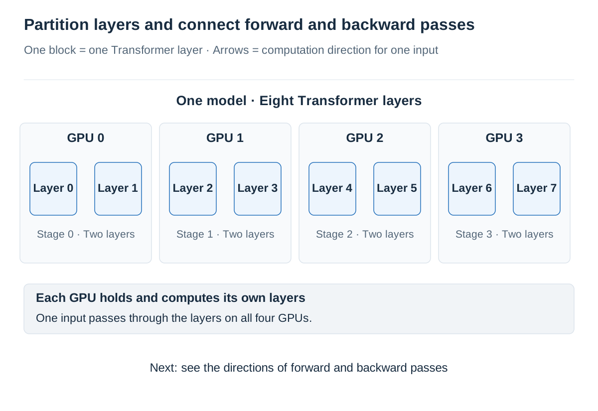
Consider a model with eight Transformer layers. GPU 0 handles layers 0 and 1, GPU 1 layers 2 and 3, GPU 2 layers 4 and 5, and GPU 3 layers 6 and 7. Each group of layers assigned to a GPU is a pipeline stage. Here, each stage uses one GPU. We omit the remaining input and output components to focus on the connections between these eight layers.
Computation from input to output is the forward pass. Once GPU 0 computes the first two layers, it sends their output activations to GPU 1. GPU 1 uses those values to compute the next two layers, continuing this way through GPU 3. Rather than moving weights to the next GPU each time, weights stay at their stages while intermediate values move.
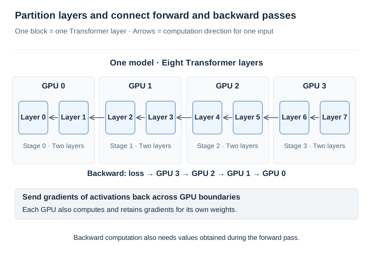
During training, the model’s output and the target are used to compute a loss, a value representing error. The backward pass retraces the computation toward earlier layers, computing gradients that describe how each value affects the loss. Use Next in the figure to compare the forward and backward directions.
Place eight layersView the completed figure
Use Next to follow the computation. Click the figure to enlarge it.
The backward pass proceeds from GPU 3 toward GPU 0. For example, GPU 1 backpropagates through its layers using gradients received from the later stage and values obtained during the forward pass. It computes gradients for its own weights locally and sends gradients of its input activations to the preceding stage, GPU 0. The reverse arrows show these activation-gradient transfers.
Either direction requires the results of preceding computations. In a forward pass for one input, GPU 1 cannot begin before GPU 0 has produced the activations. Multiple GPUs do not compute all layers of the same input simultaneously. Let us see what waiting this dependency creates when several inputs are executed together.
Waiting when the whole batch is passed onward
A batch is a group of inputs processed together. If input sequences A, B, C, and D form one batch, its batch size is four. Each input contains multiple tokens.
First, assume that all four inputs are computed as one group and that their results are passed to the next GPU together. While GPU 0 computes A, B, C, and D, GPU 1 waits for its input. So do GPU 2 and GPU 3. GPU 1 can start only after GPU 0 finishes computing the whole batch.
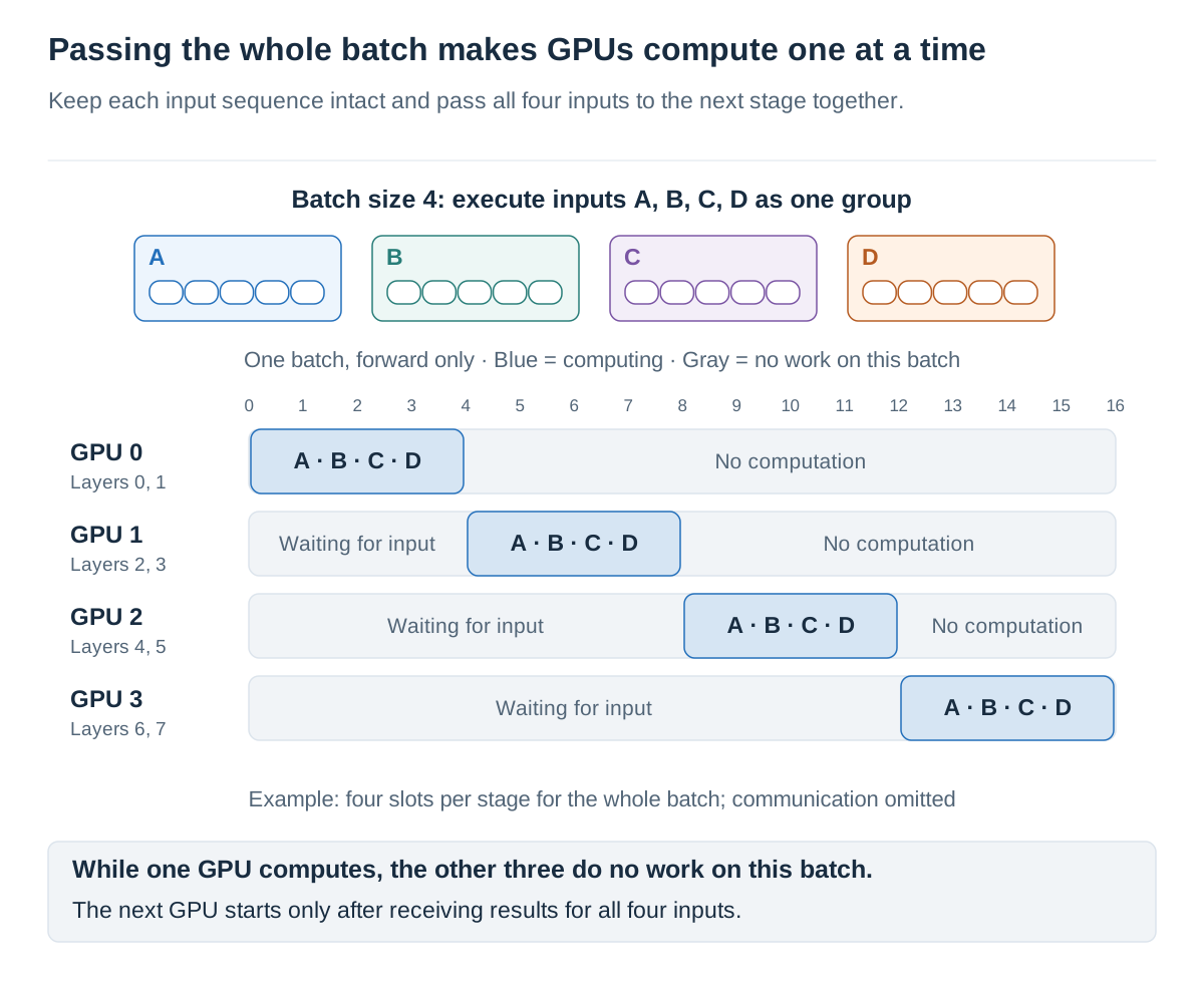
In the figure, even after GPU 1 starts computing, GPU 2 and GPU 3 still wait, while GPU 0 has already finished its own computation. With only this batch running, one GPU computes while the other three have no computation to perform. The layers are distributed, but computation still proceeds one GPU at a time.
Could the next GPU start sooner? Instead of waiting until all four inputs have been computed, send A’s result to the next GPU as soon as A is ready. This requires executing the batch in smaller groups.
Split the batch to start the next GPU sooner
A microbatch is a smaller group formed by splitting that batch. Here, we place A, B, C, and D in separate microbatches of size one: a batch of size four executed as four groups of size one. There are still four inputs, and each input’s token sequence remains intact.
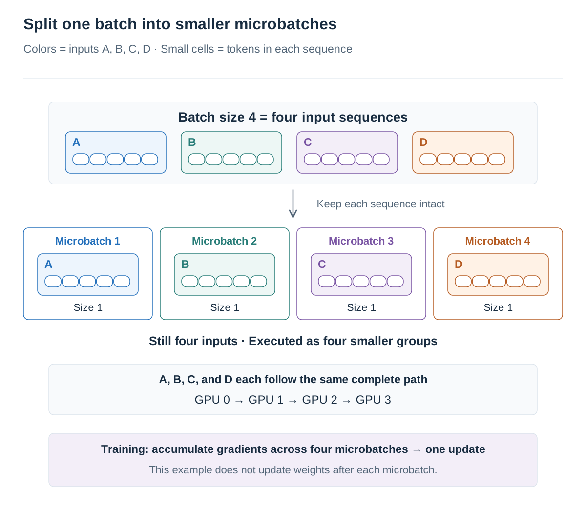
This does not mean assigning A to GPU 0 and B to GPU 1 and stopping there. Each GPU holds only some model layers, so A, B, C, and D must all pass through GPU 0 to GPU 3. What changes is the size of the group passing through each stage. Size one is only an example; a batch of size eight could instead be split into four microbatches of size two.
For training, distinguish splitting execution into smaller groups from changing how often weights are updated. This article assumes a configuration that uses the same weights throughout the four microbatches’ forward and backward passes, accumulates gradients for the whole batch, then updates the weights once. This is the approach described in the GPipe paper. It does not turn the batch into four training steps that update weights after each input.
Overlap computation for different inputs
When the batch is passed as a whole, GPU 1 waits until GPU 0 has computed all four inputs. With microbatches, GPU 0 can send A’s result to GPU 1 as soon as A is ready. While GPU 1 computes A, GPU 0 computes B. Each input retains its computation order, while computations for different inputs overlap.
Compare these executions using the same four GPUs and the same four inputs. To make the difference clear, assume that each stage takes one time slot to compute one input and four slots to compute the whole batch of four. All stages take the same time, and communication time is omitted. The next figure compares forward passes only under these assumptions; it does not show total training time including backpropagation.
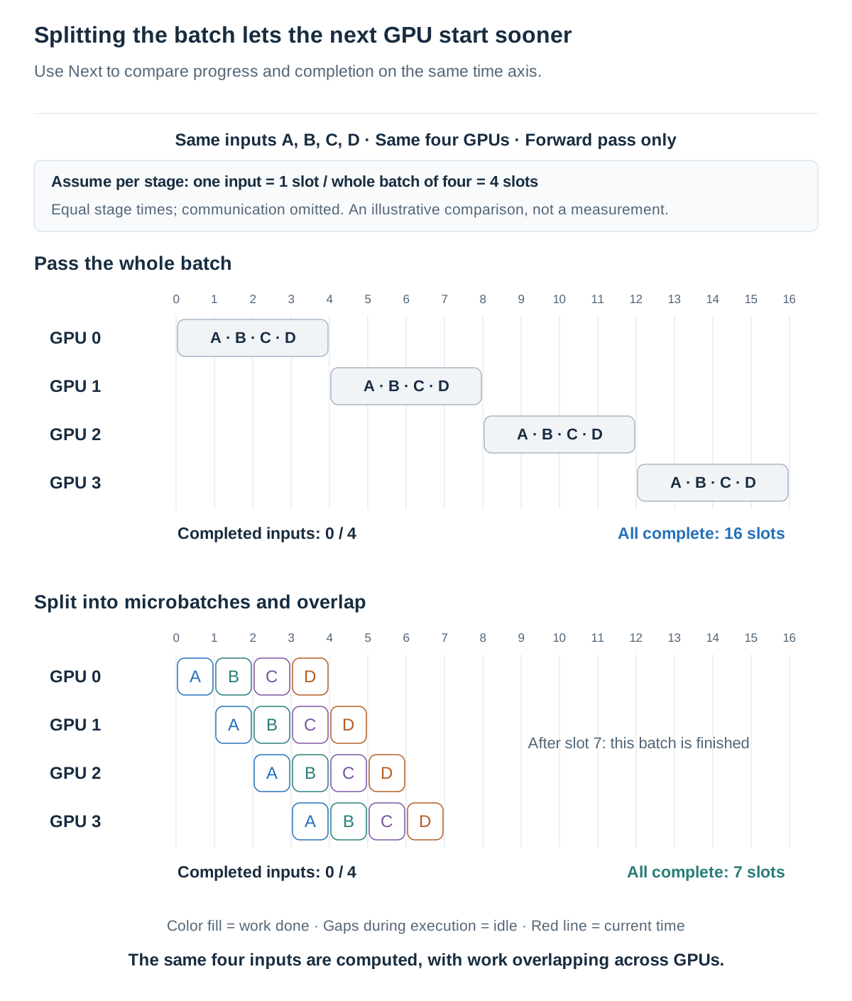
Before executionView the completed figure
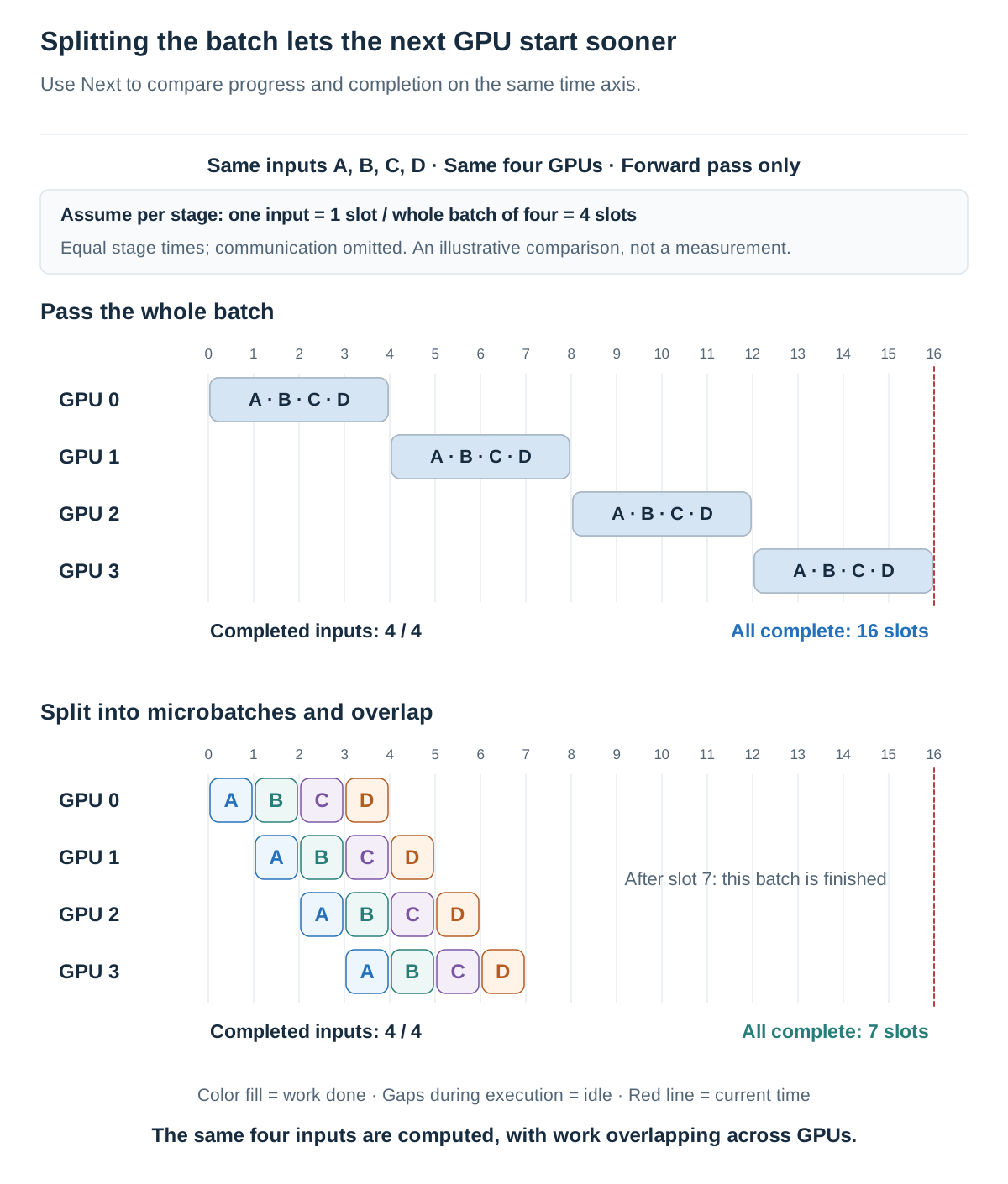
Use Next to follow the computation. Click the figure to enlarge it.
At the top, GPU 0 computes the entire batch for four slots. GPU 1 then receives the result and computes for another four slots, followed by GPU 2 and GPU 3. All four inputs finish passing through the last GPU after 16 slots. Each GPU’s block represents processing all four inputs together.
At the bottom, GPU 0 passes A to GPU 1 after one slot. During the next slot, GPU 0 computes B while GPU 1 computes A. As later stages fill, the interval from time 3 to 4 has GPU 0 computing D, GPU 1 computing C, GPU 2 computing B, and GPU 3 computing A simultaneously. A finishes after four slots, and all inputs, including D, finish after seven.
In this example, finishing the same four inputs in seven slots instead of 16 increases throughput. Throughput is the amount of work completed per unit time. No input skips required layers, and no computation is removed. Each GPU performs four slots of computation in either case; what changes is the time spent waiting for other GPUs.
In practice, computing a batch of size four does not necessarily take exactly four times as long as computing a batch of size one. Larger-batch matrix operations may be more efficient, and transferring microbatches also costs communication time. The 16-versus-seven comparison therefore illustrates how sending smaller groups onward lets the next GPU start sooner, rather than guaranteeing an actual speedup.
Balance remaining waits against microbatch size
The microbatch diagram still contains gaps. Initially, later GPUs wait for A to reach them. At the end, earlier GPUs become idle after D leaves them, while D continues through later stages. These empty periods while filling and draining the pipeline are called bubbles. At the bottom of the figure, the interval after slot seven is already past the end of this batch’s forward pass.
Sending more microbatches through the pipeline can reduce the fraction spent waiting at the start and end. But splitting a fixed batch too finely makes individual matrix operations smaller, potentially reducing GPU efficiency while increasing the number of transfers and the cost of managing execution. More microbatches do not always mean faster execution.
Unequal stage times introduce additional waiting around a slow stage. Assigning two layers per GPU does not guarantee equal execution times. In practice, each stage’s computation, memory usage, and data transferred across its boundaries must be considered together.
Inference can also overlap different inputs across stages. However, when a request generates tokens one at a time, the previous token’s result is needed to determine the next input, so that dependency remains. Having enough inputs to make progress together also affects how well the pipeline can be filled.
PP distributes model layers across GPUs and uses microbatches to overlap computation for different inputs.