Attention and MLP: Information Across Tokens and Transformations Within a Token

In the previous article, we divided a decoder block into the residual stream and the transformation paths alongside it. Each side path computes the output of Attention or MLP after RMSNorm, then adds that result to the residual stream. In this article, we will compare the roles of Attention and MLP, which we previously showed as faded boxes, and explore the computations inside an MLP.

Which tokens do Attention and MLP use?

Attention and MLP both transform token vectors, but they differ in whether they refer to vectors at other token positions. Attention brings information from other positions into the vector at the current position. MLP, on the other hand, operates independently on each token’s vector. The figure below compares which inputs contribute to the output for the third token.

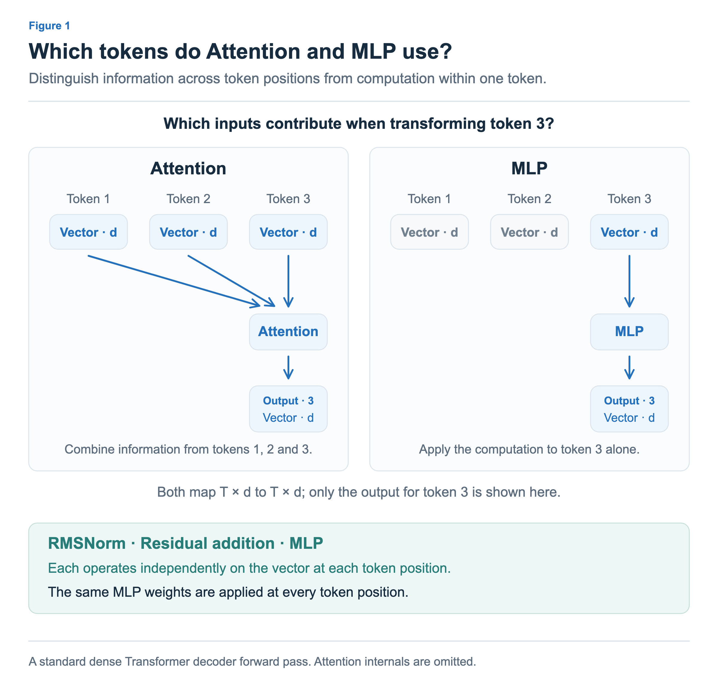
On the left, Attention uses the vectors for tokens 1 and 2, as well as token 3’s own vector, to compute the output vector for token 3. This incorporates surrounding context into its vector. On the right, MLP takes only token 3’s vector and computes an output vector at the same position. The figure shows only the output for token 3, but the full input and output shapes of both transformations are T × d.

In the forward pass of the basic Transformer decoder we are discussing, Attention combines information from different token positions. RMSNorm normalizes over the d components of one token, residual addition adds vectors at the same position, and MLP transforms one token’s vector. The same MLP weights are applied at every token position.

Matrix multiplication: Combining input components to produce outputs

Before looking inside MLP, we will examine matrix multiplication, which it uses. Multiplying a token vector, written as a row, by a learned weight matrix produces a new vector. If the input has d dimensions and the weight matrix has shape d × m, the output has m dimensions. Here, m is the intermediate dimension used inside MLP. The figure uses a small example with d = 4 and m = 8.

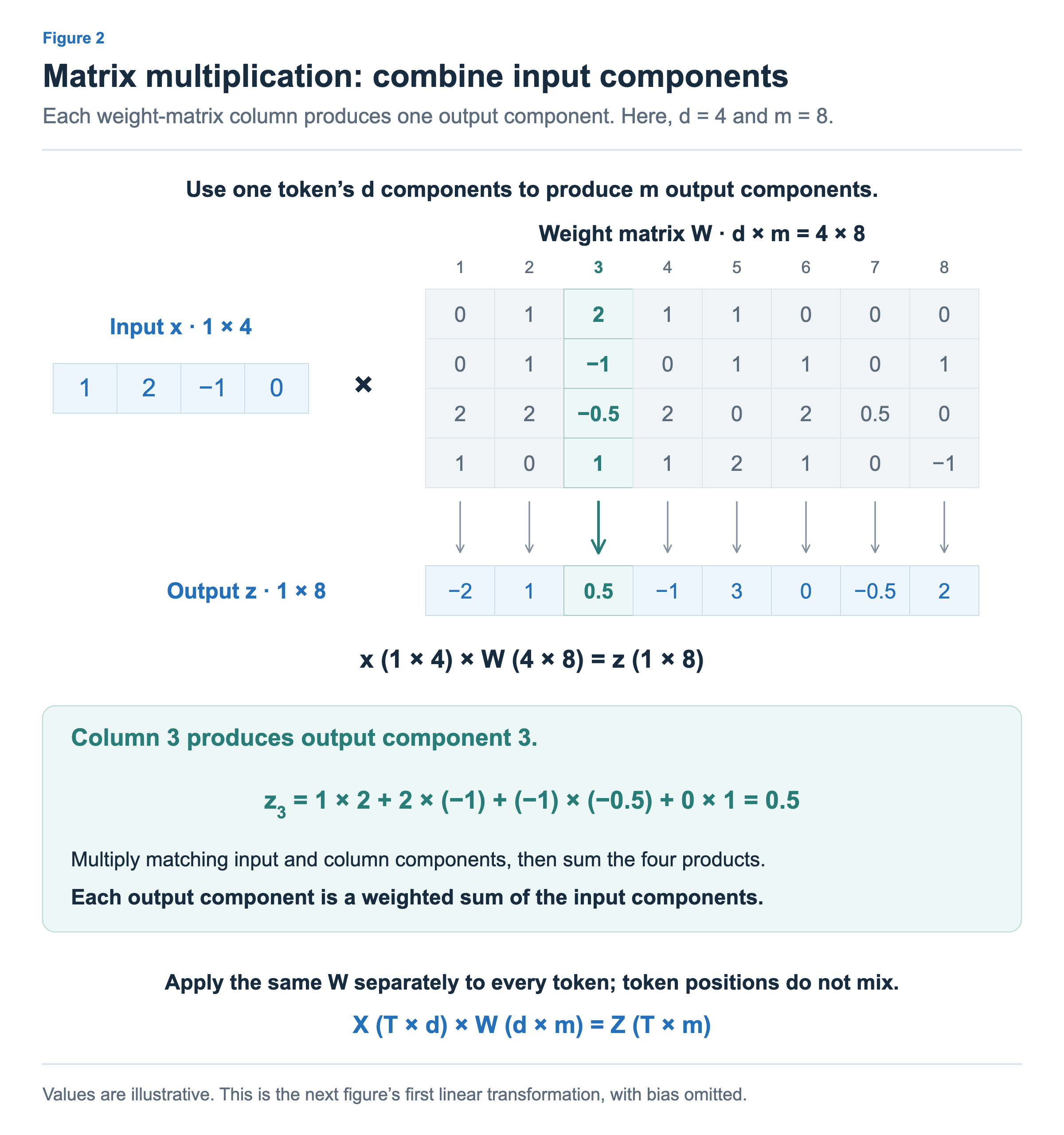
Each output component is computed using the input vector and one column of the weight matrix. Multiply corresponding values, then add all the products. For example, if the input is [1, 2, −1, 0] and the third column is [2, −1, −0.5, 1], the third output is 1 × 2 + 2 × (−1) + (−1) × (−0.5) + 0 × 1 = 0.5. Repeating this for all eight columns produces eight output components. Each column combines the input components with a different set of weights.

This computation combines components within one token’s vector. Stacking T tokens as rows lets us write the computation as X (T × d) × W (d × m) = Z (T × m). Each output row is still computed from its corresponding input row and the same weight matrix W. Computing multiple tokens together as a matrix does not mix information across tokens. The weights and dimensions in the figure are illustrative, and we omit bias to keep the computation simple.

Basic MLP: Expand → Activate → Reduce

MLP stands for Multi-Layer Perceptron and is also called an FFN (Feed-Forward Network) in Transformers. Its basic form places an activation function between two linear transformations. First, matrix multiplication expands a d-dimensional vector to a larger m-dimensional vector. An activation function is applied, then a second matrix multiplication maps it back to d dimensions. The first linear transformation below uses the same values as the preceding matrix multiplication example.

The first transformation produces [−2, 1, 0.5, −1, 3, 0, −0.5, 2]. Applying ReLU replaces negative values with zero and leaves nonnegative values unchanged. The result is [0, 1, 0.5, 0, 3, 0, 0, 2]. The activation function operates on each component without changing the number of components. The second linear transformation then combines these eight modified components to produce a vector with four components.

The activation function between the two linear transformations makes the overall transformation nonlinear. Without it, consecutive matrix multiplications could be combined into a single linear transformation by multiplying the two weight matrices in advance. Inserting a function such as ReLU, whose behavior depends on the input value, allows MLP to learn a wider range of transformations. Although the dimension expands internally, the final output returns to d dimensions, so it can be added to the residual stream at the same token position.

Gated MLP: Compute along two branches, then multiply

Building on the basic MLP, we have Gated MLP. Here we will examine SwiGLU, which uses the SiLU activation function. The same input x branches into two paths: Up projection produces an intermediate vector u, while Gate projection followed by SiLU produces a vector g. The two projections receive the same input but use different weights.

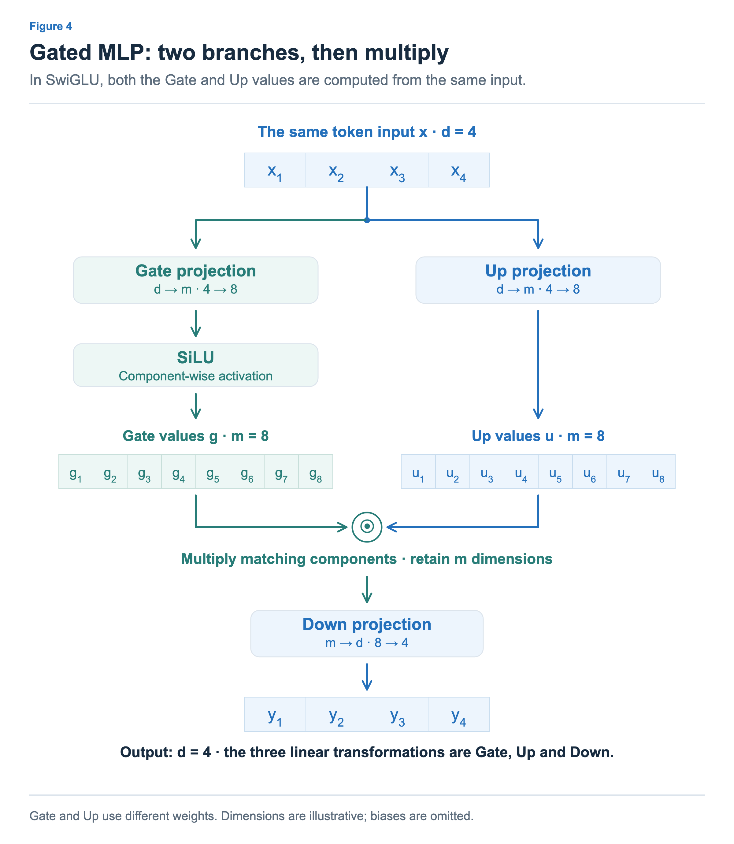
Both branches produce m-dimensional vectors. Their corresponding components are multiplied, then Down projection maps the result back to d dimensions. The symbol ⊙ denotes this component-wise multiplication. There are three linear transformations—Gate, Up, and Down—but the input does not pass through three layers in sequence. Gate and Up branch from the same input; their results are multiplied before reaching Down. This structure and the definition of SwiGLU are presented in GLU Variants Improve Transformer.

SiLU is an activation function that multiplies each input value by its sigmoid. For this article, we will focus on the component-wise activation in the Gate path and the multiplication of its result with the Up path’s values, rather than the detailed curve. As in the basic MLP, the entire computation takes place within one token, and both input and output have d dimensions.

Gate: Adjusting each component based on the input

We can understand the Gate as adjusting how much of each value from the Up path is passed on. From the same input, Up computes the values to adjust, and Gate computes their multipliers. These multipliers are computed from the current input rather than being fixed constants, so they change with the input. The figure below zooms in on four components of the intermediate vector.

The first component shrinks to 2 × 0.1 = 0.2, while the second grows in absolute magnitude to −1 × 1.5 = −1.5. The third becomes zero, and the fourth grows to 0.5 × 2 = 1. The Gate values shown are after SiLU. SwiGLU’s Gate values are not restricted to the range from 0 to 1. They can exceed 1 or be negative, so a multiplier that can reduce or increase a value and change its sign is a more accurate description than an on/off switch.

An activation function already adjusts component values in a basic MLP. Gated MLP differs by using a separately learned path to compute the multipliers alongside the values they adjust. This is an intuition for the computation that a Gate makes possible. Quality improvements must be established experimentally: the SwiGLU paper reports lower perplexity than the ReLU-based FFN in a comparison matched for parameter count and computation. The figures use the same intermediate dimension to compare the structures, but actual models choose this dimension according to their design.

We can now distinguish the two main transformations in a decoder block. Attention combines information across tokens, while MLP transforms the components within each token. A basic MLP expands, activates, and reduces; a Gated MLP includes component-wise multiplication of two vectors computed from the same input. In the next article, we will look inside Attention, starting with the projections that turn input vectors into Q, K, and V, and the output projection that maps the Attention result back to the model dimension.