The Flow Through a Decoder Block: Residual Connections and RMSNorm

In the previous article, we divided the overall structure of an LLM into the embedding layer, decoder blocks, and the LM Head. We also saw that a decoder block takes T token vectors, each with d dimensions, and returns vectors with the same T × d shape. In this article, we will look inside the decoder block that we previously drew as a single box. We will start by distinguishing the main path that carries the vectors from the computations that branch off and then rejoin it.

Viewing a Decoder Block Around the Residual Stream

We can broadly divide a decoder block into the residual stream, RMSNorm, Attention, and MLP.

Decoder block diagrams commonly place Attention and MLP in the center, as on the left below, with lines around the outside carrying the input past each transformation and back to an addition. This time, we will place the path carrying the input vectors in the center, with Attention and MLP on side branches, as on the right. This central path is called the residual stream. At each split, the input passes unchanged along the central path, while the side branch uses that input to compute a transformation result. Where the two paths meet, the result is added to the input, and the sum continues to the next computation.

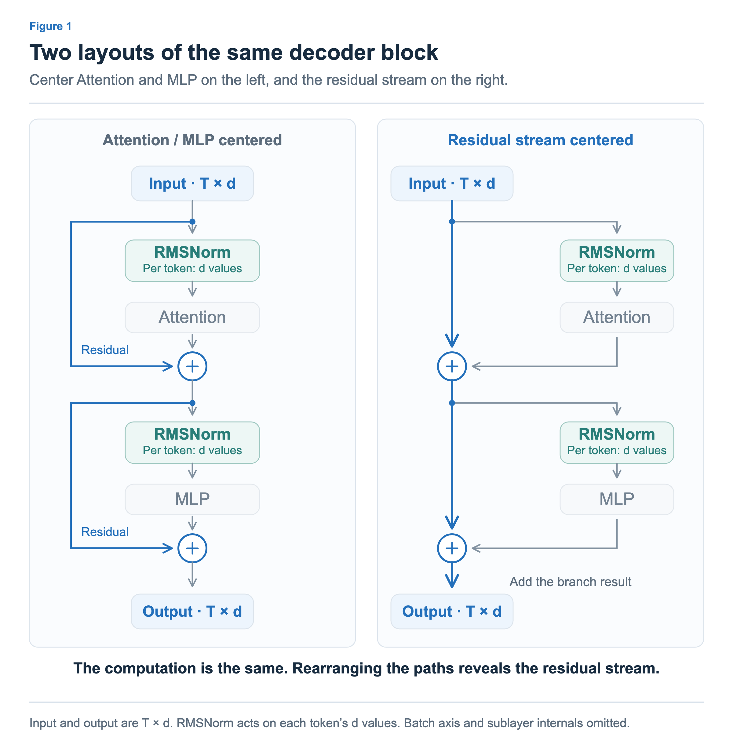
Following the right-hand diagram from top to bottom, the first side branch applies RMSNorm and Attention, and its result is added to the central stream. The second side branch applies RMSNorm and MLP, and its result is added in the same way. Attention and MLP perform the main transformations, and their results are added to the residual stream. Their boxes are muted so that we can see where they sit without looking inside them yet. In this article, we will first examine the residual stream and the RMSNorm operations on its side branches.

Residual Connections: Adding an Update to the Input Vector

A residual connection adds a transformation result to the input that has been passed through unchanged. If the input is x and the result computed by the side branch is Δ, the output is x + Δ. Vector addition combines components at matching positions: the first components are added together, then the second components, and so on. The input and the result being added must therefore have the same dimensions. If one token’s input vector has d dimensions, the update also has d dimensions, and so does their sum.

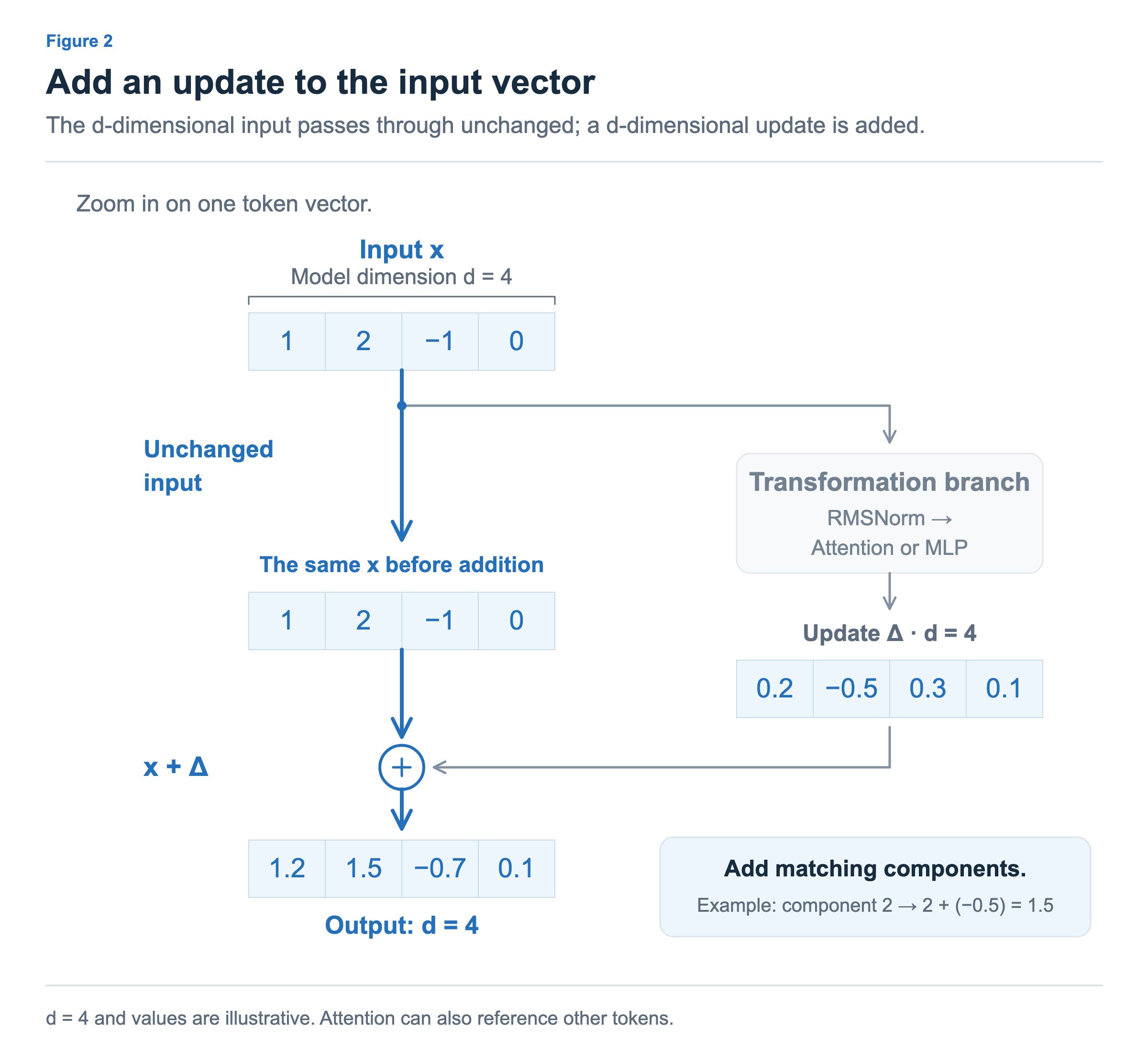
The diagram zooms in on one token vector. If the input is [1, 2, −1, 0] and the update is [0.2, −0.5, 0.3, 0.1], the output is [1.2, 1.5, −0.7, 0.1]. For example, the second component is calculated as 2 + (−0.5) = 1.5. The input retains the same values until the addition; after the paths merge, their sum continues along the next path. The dimensions stay the same while the component values change. Across all tokens, this operation adds two T × d arrays at matching positions. The numbers in the diagram are illustrative, and Attention can also reference other token vectors when computing its update.

RMSNorm: Adjusting Scale Across a Token’s d Components

A vector entering a side branch goes through RMSNorm before being passed to Attention or MLP. RMS stands for Root Mean Square: square the components, take their mean, and then take the square root. For a token vector with d components, these d values produce one RMS. Dividing each component by that same RMS adjusts the vector’s scale.

RMSNorm includes one more step. After division by the RMS, the result is multiplied component by component by a learned weight vector, γ (gamma). If the input has d dimensions, γ also has d values, each adjusted during training. In the diagram below, we set γ to [1, 1, 1, 1] to focus first on the effect of dividing by the RMS. Multiplication by 1 leaves a value unchanged, so the output in this example is simply the result of that division.

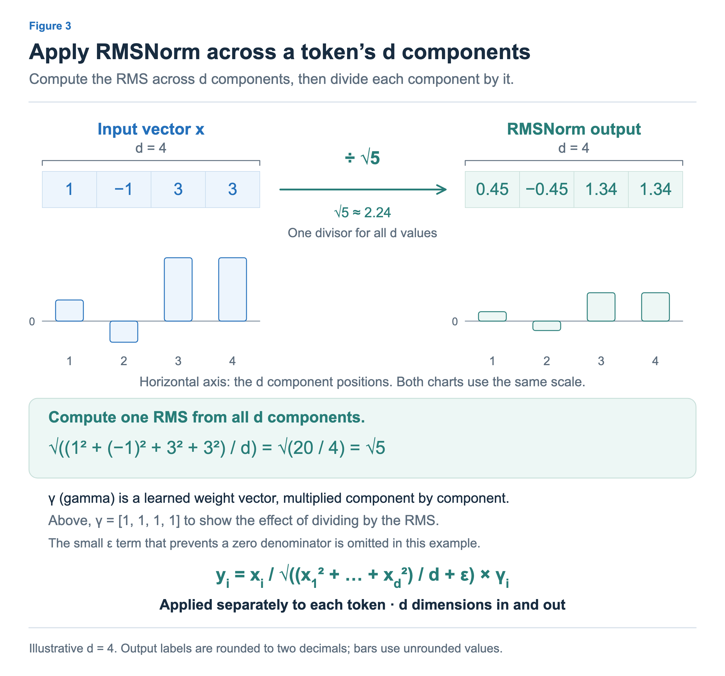
For the input [1, −1, 3, 3], the sum of squares is 1 + 1 + 9 + 9 = 20. There are d = 4 components, so the mean square is 5 and the RMS is √5 ≈ 2.24. Dividing each component by √5 gives approximately [0.45, −0.45, 1.34, 1.34]. Both charts use the same scale, making it possible to compare how the magnitude of each value changes. To keep this calculation simple, the example omits the small value ε (epsilon). The full formula adds ε inside the square root to prevent a zero denominator.

The RMS is computed across the d components of one token. With T tokens, an RMS is computed separately for each token vector. The same RMSNorm layer uses the same γ for all tokens, but the RMS divisor depends on each token’s vector. The number of components does not change, so the input and output both have shape T × d. In Figure 1, this normalized value is passed to Attention or MLP, while the central path retains the value from before normalization until the transformation result is added.

Locating RMSNorm in the Overall Model

We can now add RMSNorm to the overall structure from the previous article. Besides the RMSNorm operations inside the decoder blocks, one more RMSNorm sits between the final decoder block’s output and the LM Head. It normalizes each token’s d-dimensional vector from the final block before the LM Head converts it into vocabulary scores.

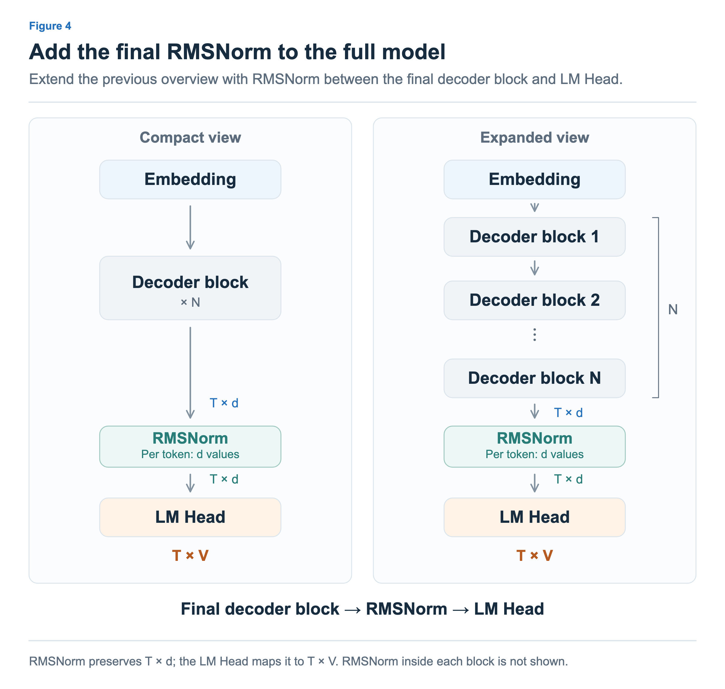
We can now view the decoder block as a residual stream with transformation branches beside it. The residual stream carries each branch’s input unchanged, adds the transformation result where the paths rejoin, and passes the sum to the next stage. Each side branch applies RMSNorm and then computes an Attention or MLP result. In the next article, we will compare the roles of Attention and MLP, which we have kept as muted boxes here, and examine the computations inside the MLP.