Why Attention Is Difficult to Optimize

In the previous article, we explored how to save time by reusing matrix multiplication inputs and overlapping data movement with computation. Now we turn to Attention. Between its two matrix multiplications, Attention produces large score and probability matrices. Storing these intermediate results in global memory and rereading them for the next computation can take substantial time. Reducing Attention’s execution time therefore requires examining both matrix multiplication speed and the movement of intermediate results.

What if we computed scores a few at a time, immediately converted them into probabilities, and used them in the next computation? This runs into a difficulty: a subset of scores is not enough to determine their final probabilities. In Softmax, even one probability depends on the other scores in the same row. We will first examine why storing and rereading intermediate matrices is costly, then see where difficulties arise when we try to reduce that traffic by continuing computation tile by tile.

The Attention Computation Flow

Let us briefly revisit the computation from the Core Attention article. We consider one head processing T tokens together. If the dimension of one head is dₕ, Q, K, and V each have shape T × dₕ.

A row of Q is the Query vector of a token gathering information, and a row of K is the Key vector of a token it can attend to. Their dot product gives one score between tokens. Computing these scores through matrix multiplication QKᵀ produces a T × T score matrix S, with rows corresponding to Query tokens and columns to Key tokens.

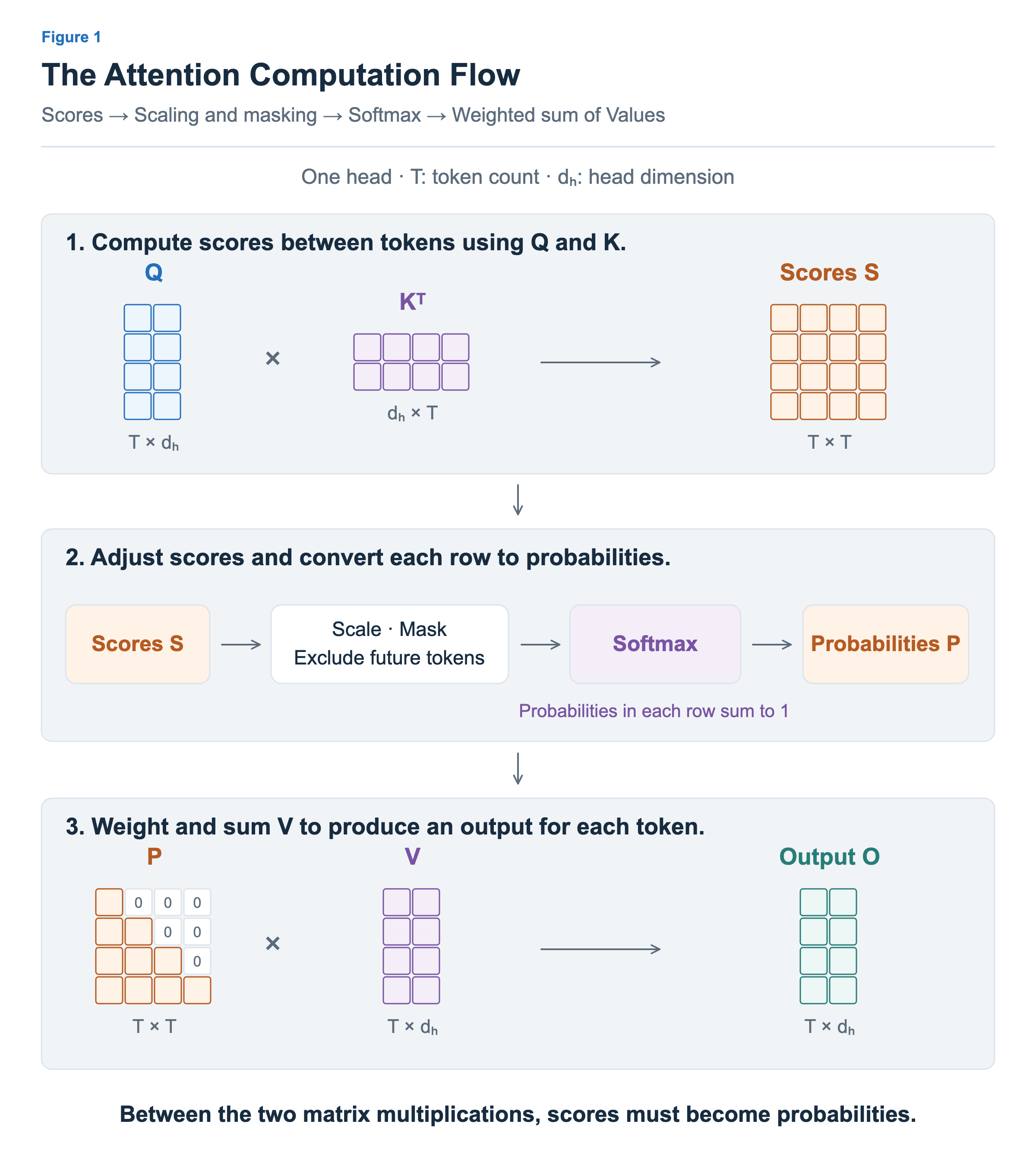
The second stage in Figure 1 divides the scores by √dₕ to adjust their scale and masks positions that cannot be attended to. Here we use a causal mask, so each token can attend only to itself and earlier tokens. Setting scores for future tokens to −∞ makes their Softmax probabilities zero.

Softmax then converts the scores in each row into probabilities that sum to 1. These probabilities are the weights that determine how much each token’s Value contributes. Each score has a corresponding probability, so the probability matrix P also has shape T × T.

Finally, multiplying P by V produces output O. For each Query token, a probability-weighted sum of Value vectors gives dₕ components. The full output has shape T × dₕ. Attention thus starts with T × dₕ inputs, passes through T × T intermediate matrices, and produces a T × dₕ output.

Storing and Rereading Large Intermediate Matrices

Suppose we run these computations separately and store their intermediate results in global memory. The kernel computing QKᵀ stores the score matrix S and finishes. The next kernel reads S, performs scaling, masking, and Softmax, and stores the probability matrix P. The final matrix multiplication reads P and multiplies it by V.

Values needed by the next kernel must remain available after the current kernel ends. The registers or a block’s shared memory used by one kernel cannot simply be handed to the next kernel, so this implementation puts intermediate tensors in global memory. In Figure 2, downward arrows show results being stored, and upward arrows show the next computation rereading those results.

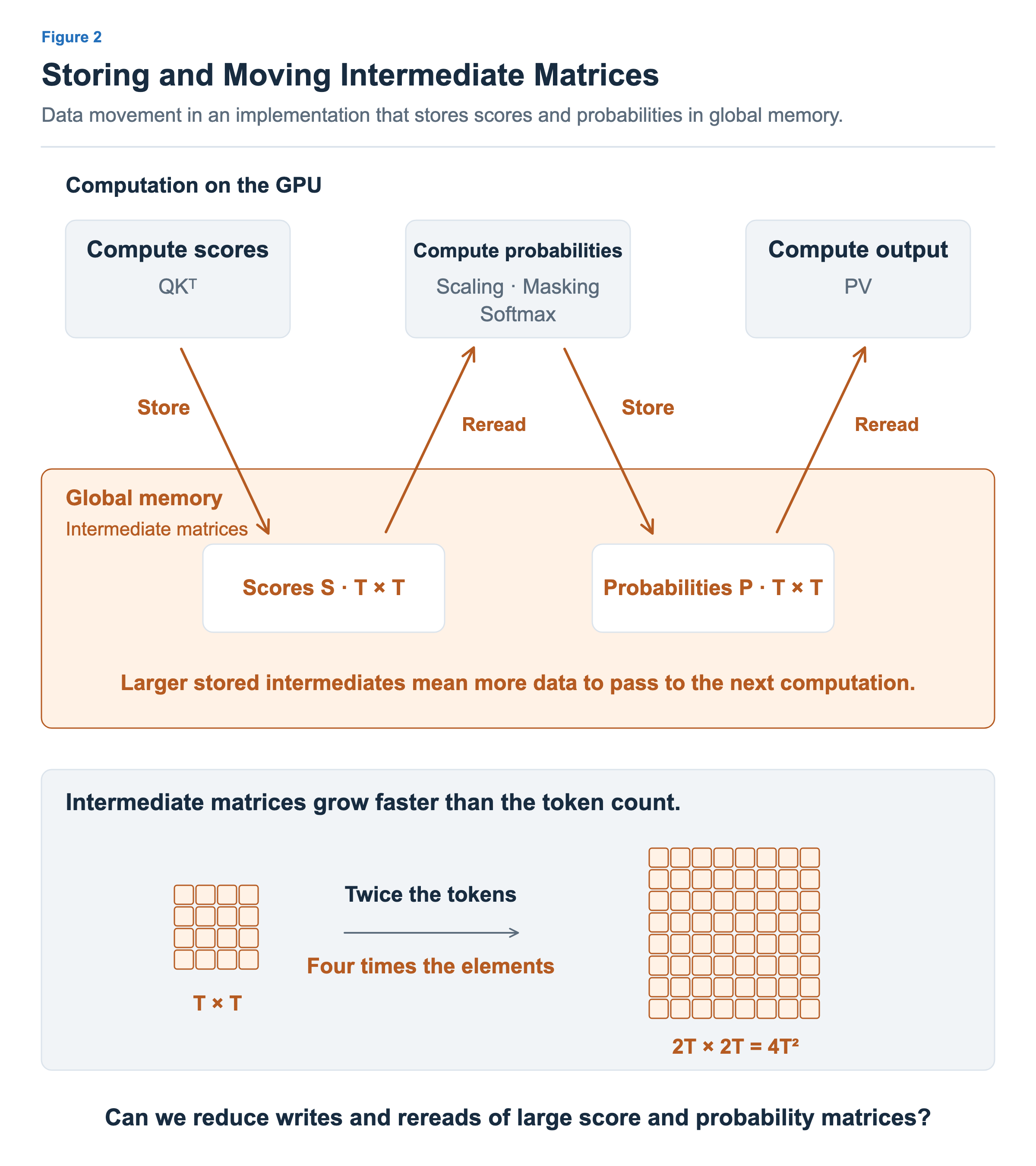
S and P each contain T × T values. Doubling the token count doubles both the rows and columns, quadrupling the number of elements in each matrix. For example, with T = 4,096 and 2 bytes per value, one matrix occupies 32 MiB. With T = 8,192, a matrix in the same format occupies 128 MiB. A MiB is 1,048,576 bytes.

This size affects more than storage capacity. Every time a large matrix is stored and reread, that amount of data must be transferred. The figure shows S being stored and read, followed by the same sequence for an equally large P. Large amounts of data move repeatedly just to pass temporary intermediate results to the next stage.

Caches participate in global memory accesses, so not every read or write corresponds one-to-one with an actual HBM transfer. But as intermediate matrices grow too large for caches alone to handle the handoff, traffic to and from HBM also grows. HBM bandwidth is limited, so more traffic means more time is needed to store and supply the data. In particular, the scaling, masking, and Softmax stage reads, processes, and rewrites a large matrix, making data movement a potentially large part of its execution time. Standard Attention implementation analysis in the original FlashAttention paper

In the previous article, we used tiling to reuse inputs within a matrix multiplication. Now, to reduce the cost of storing and reading S and P between the two matrix multiplications, we will explore how to keep the values produced by one computation in nearby memory and use them in the next computation.

From a Score Tile to Probabilities

For element-wise operations, we previously examined fusion: combining multiple computations into a single kernel. Proceeding directly to the next computation on the same element reduced the need to store an intermediate value in global memory and reread it. In Attention, computing a small score tile and immediately using its values in the next stage could similarly reduce the need to store and reread the full score matrix in global memory.

Figure 3 shows the scores for query tokens 2 and 3 against key tokens 0 and 1 being computed first, with T = 4. Token indices start at 0 here. Selecting two rows of Q and two columns of Kᵀ and multiplying them produces a 2 × 2 score tile. Each of the four scores in the tile has a fully completed dot product. What remains uncomputed is not the remaining components of these scores, but the scores against other key tokens.

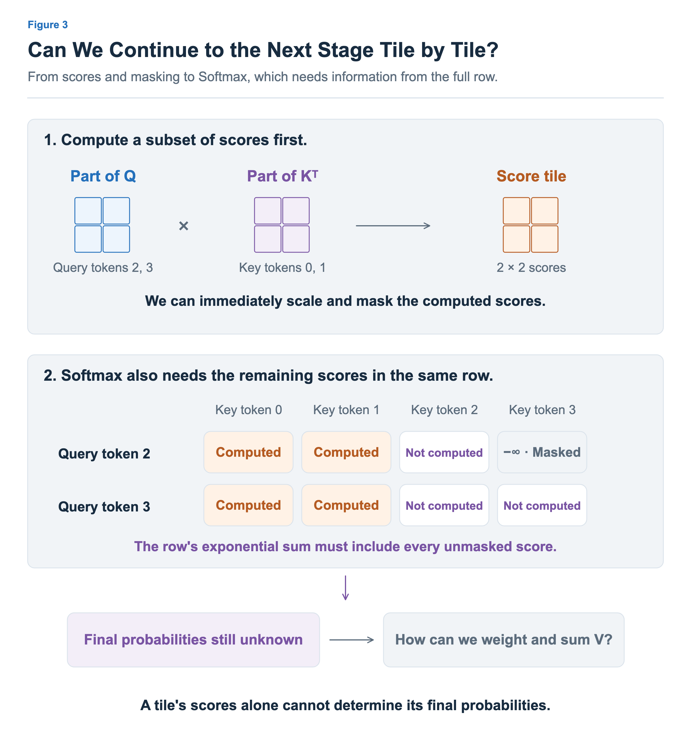
The computed scores can immediately be divided by √dₕ. Masking can also be decided using the query and key token indices at each position. Determining whether a token is in the future does not require other score values. Scaling and masking can therefore be handled immediately within the current tile.

Softmax is different. Each probability is the exponential function exp applied to its score, divided by the sum of exp applied to every unmasked score in the same row. We will call this the exponential sum. Every probability in a row uses the same exponential sum as its denominator.

Consider the row for query token 2 in Figure 3. The scores for keys 0 and 1 have been computed, but the score for key 2 is still unknown. Key 3 is a future token and is masked out. Even the probability for key 0 needs a denominator that includes the exponential of the score for key 2, as well as those for keys 0 and 1. Without the score for key 2, we cannot complete that denominator.

The row for query token 3 can attend to keys 0, 1, 2, and 3. The current tile contains only the scores for keys 0 and 1, so the scores for keys 2 and 3 must also be included before we know this row’s exponential sum. The cells labeled “Not computed” in the figure must not be treated as zeros or excluded values. These scores must also contribute to the denominator when calculating the final probabilities.

Finishing the score computation within a tile therefore does not, by itself, determine that tile’s final probabilities. All the inputs needed for each score’s dot product have been used, but information from the same row is still missing for converting that score into a probability. Scores from other query rows are not needed. The dependency spans all key positions that this query row can attend to.

This distinction carries over to the next matrix multiplication, PV. The values in P are weights multiplied by V, so an approach that finalizes weights using only the current score tile and immediately uses them runs into a problem. To continue computation, we need a way to account for how the weights change when the currently unknown scores are incorporated later.

How the Remaining Scores Change a Probability

Figure 4 illustrates this dependency with numbers. Consider a row with four unmasked positions, where the first two scores, after scaling, are 0 and 0. The last two scores have not yet been computed.

We already know the exponential of the first score: exp(0) = 1. But the probability’s denominator is the sum of the exponentials of all four scores. Knowing the numerator without knowing the denominator is not enough to determine the final probability. The figure compares two different possibilities for the unknown scores.

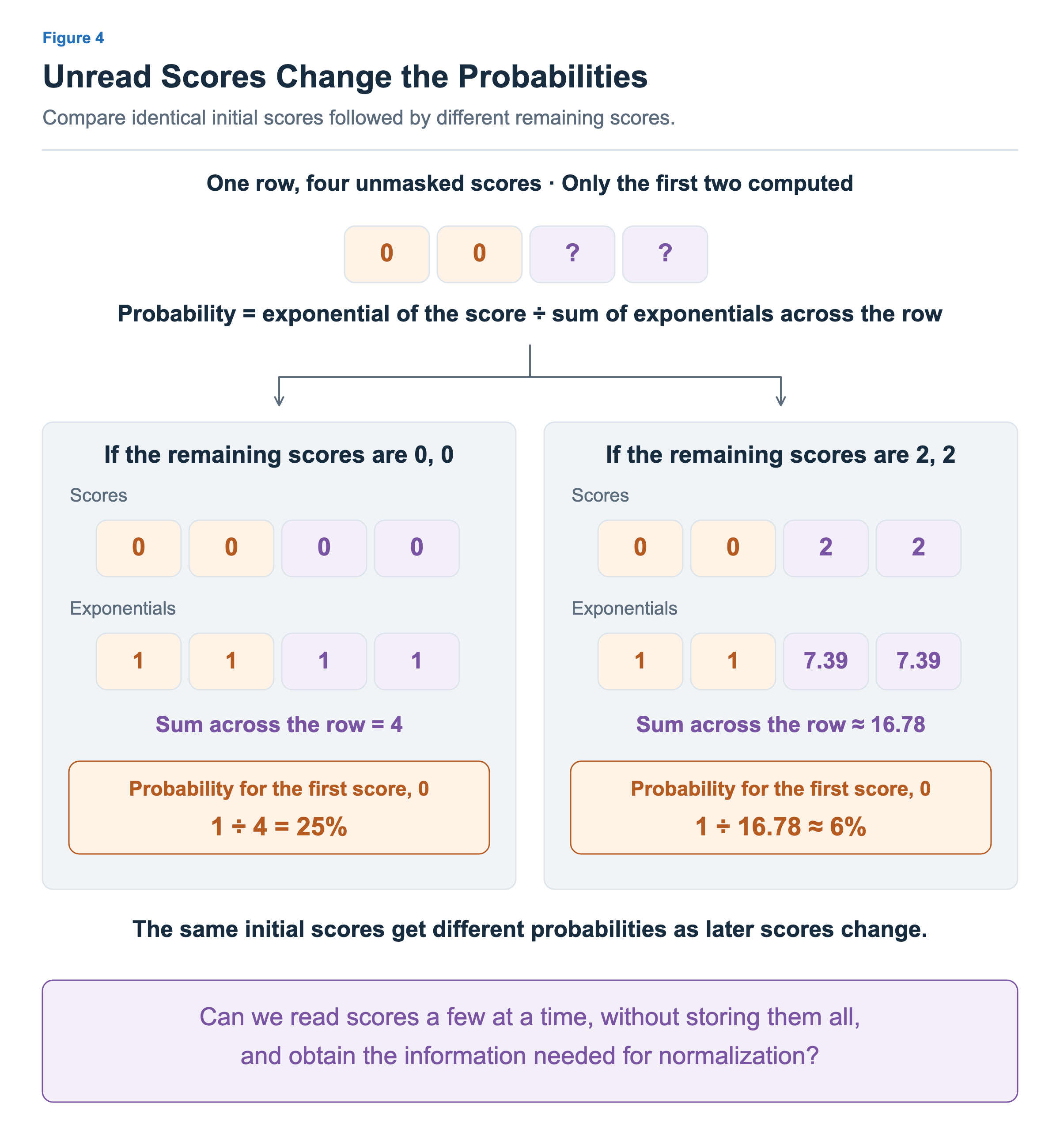
On the left, the remaining scores are also 0 and 0, giving the full row [0, 0, 0, 0]. Every exponential is 1, so their sum is 4, and the first probability is 1 ÷ 4 = 25%.

On the right, the remaining scores are 2 and 2, giving the full row [0, 0, 2, 2]. Since exp(2) is about 7.39, the exponential sum is 1 + 1 + 7.39 + 7.39 ≈ 16.78. The first probability drops to 1 ÷ 16.78 ≈ 6%. The earlier score of 0 has not changed, but the later scores increase the exponential sum and change its probability.

What if we had applied Softmax to just the first two scores? For [0, 0], the exponential sum is 2, giving 50% each. But these are probabilities normalized to sum to 1 across only the first two positions. They are not the Attention probabilities across all four positions. The first two probabilities should actually be 25% each on the left and about 6% each on the right.

Returning to Figure 3, we can now see why we cannot independently apply Softmax to each score tile and simply concatenate the results. If each tile computes a denominator using only its own scores, values in the same query row are divided by different denominators. Determining how much each Value contributes across the full row requires a common denominator that also includes unmasked scores outside the tile.

To reduce the cost of storing and rereading large intermediate matrices, we considered using results from small groups of computations immediately in the next stage. Yet a subset of scores cannot determine their final probabilities. We need a way to incorporate information from the full row. Does needing that information mean that all scores must be kept in memory at the same time?

Can we obtain the information needed for normalization by reading scores a few at a time, without storing them all? The next article will start from this question and explore online softmax.