The Structure of an LLM: From the Embedding Layer to the LM Head

In the previous article, we looked at LLM systems engineering as the work of connecting models, hardware, and workloads. We will now start with models. To understand the computations inside a model, we first need to understand how its input changes form and follows a path toward the output. This article uses a decoder-only Transformer to explain the overall structure and the roles of the embedding layer and the LM Head at either end.

The Overall Structure of a Model

We can simplify the structure of an LLM as an embedding layer → multiple decoder blocks → an LM Head. The embedding layer turns input tokens into vectors, and the decoder blocks transform those vectors in sequence. The LM Head then converts the resulting vectors into scores used to select the next token. The diagram omits details such as the final normalization to make this flow easier to follow.

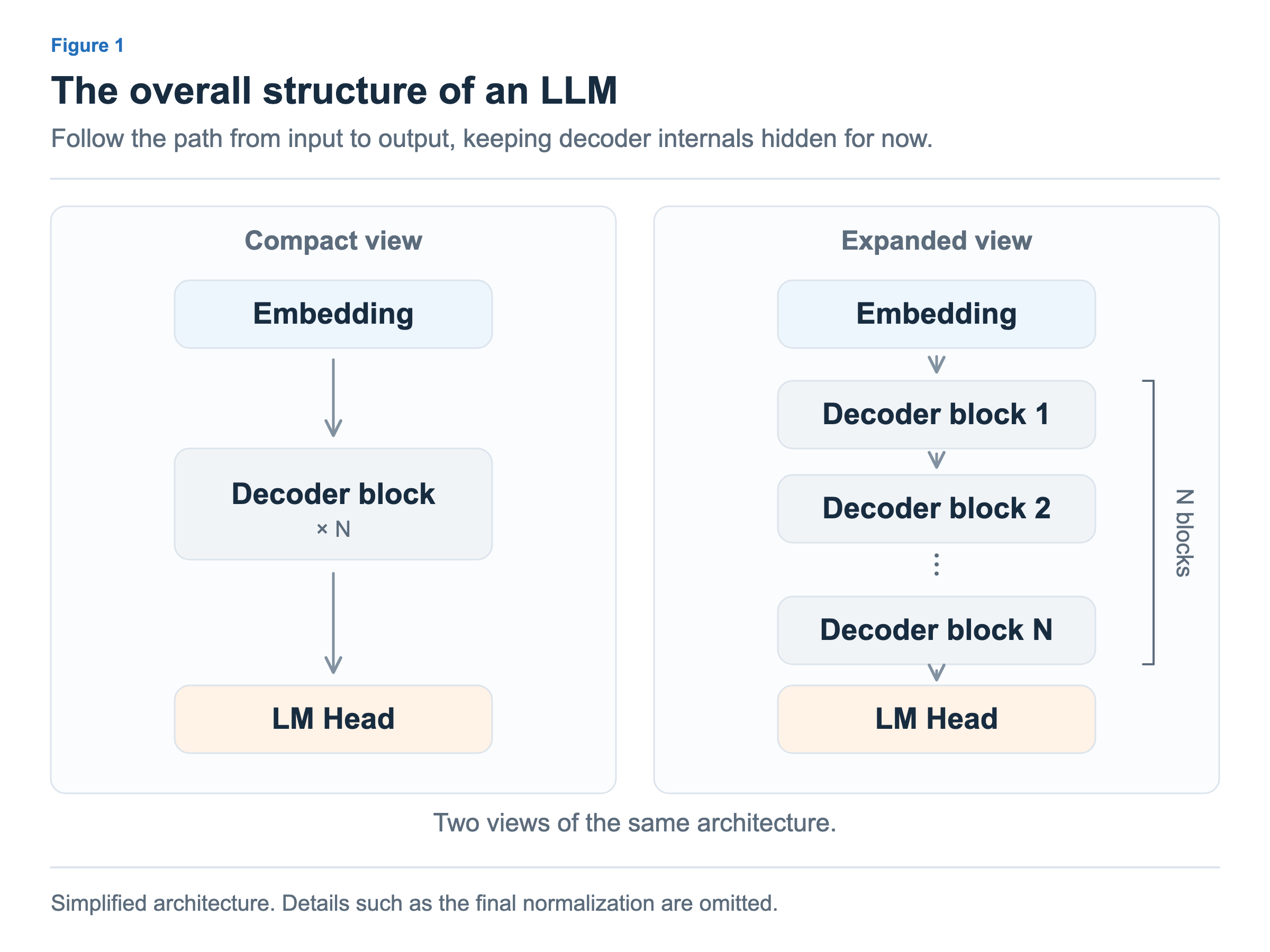
Expanding “Decoder block × N” on the left gives the sequence of blocks on the right. The output of one block becomes the input to the next. Repetition here means stacking blocks with the same structure; each block generally has its own weights. For now, we will keep the internals of each block in a single box and focus on how the inputs and outputs connect.

The Tokenizer: Converting Text to IDs

Before text enters the model, it must first pass through a tokenizer. The tokenizer splits the text into units called tokens and returns an integer ID for each token. A token may be a whole word, part of a word, or a piece containing whitespace or punctuation. How text is split and which IDs are assigned depend on the tokenizer.

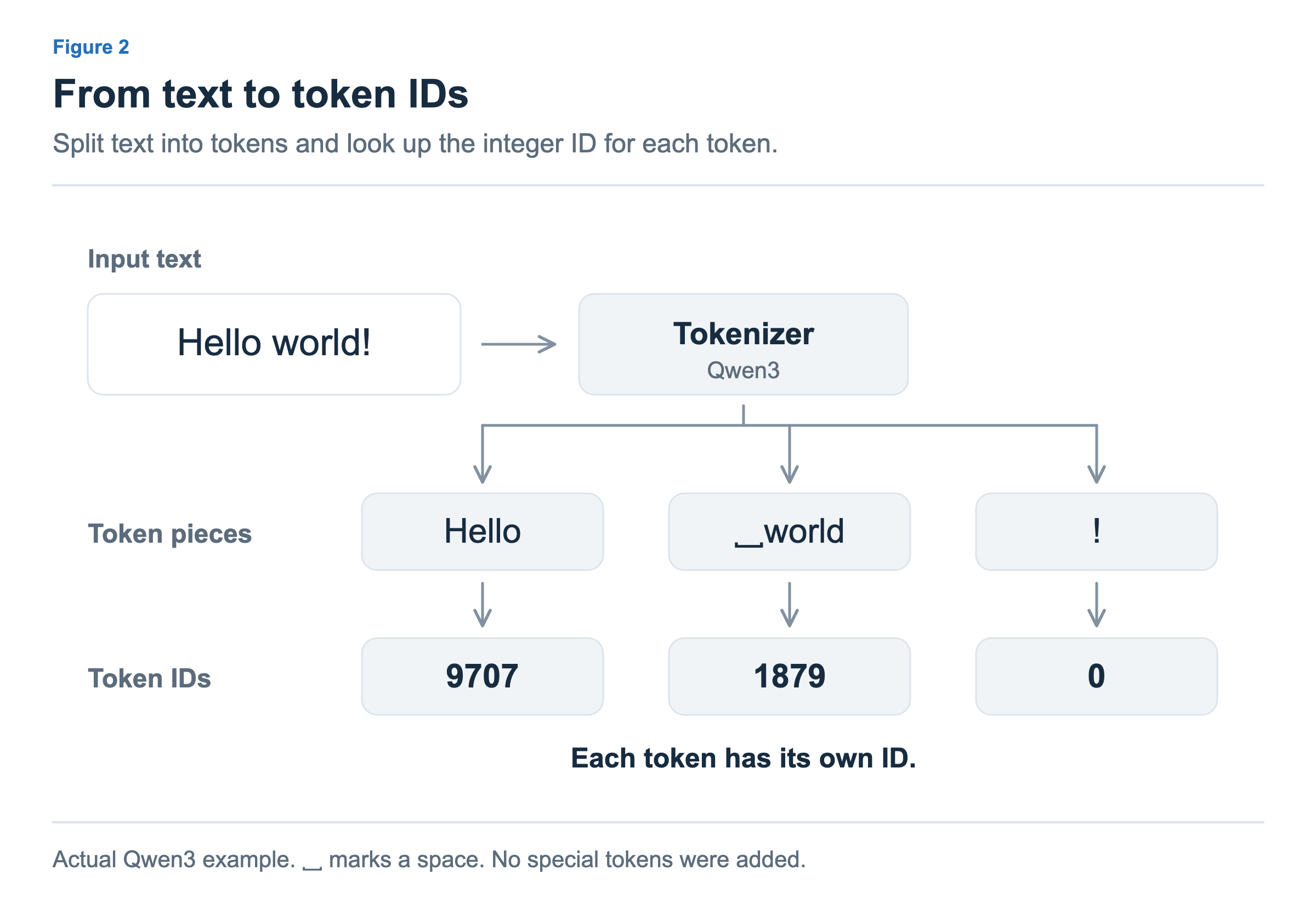
For example, the Qwen3 tokenizer splits Hello world! into Hello, world, and !, which map to IDs 9707, 1879, and 0. The ␣ symbol in the diagram makes the space before world visible. These IDs are numbers that distinguish tokens. The magnitude of an ID does not indicate the token’s meaning or importance. This list of IDs is then passed to the embedding layer.

The Embedding Layer: Looking Up a Vector for Each ID

The embedding layer retrieves the embedding vector for each token ID. A vector is an ordered list of numbers, and its dimension is the number of entries it contains. The set of tokens used by the model is called its vocabulary. If the vocabulary size is V and the model dimension is d, the embedding table has V rows and d columns. Each row stores a d-dimensional vector for its token, and these values are adjusted during model training.

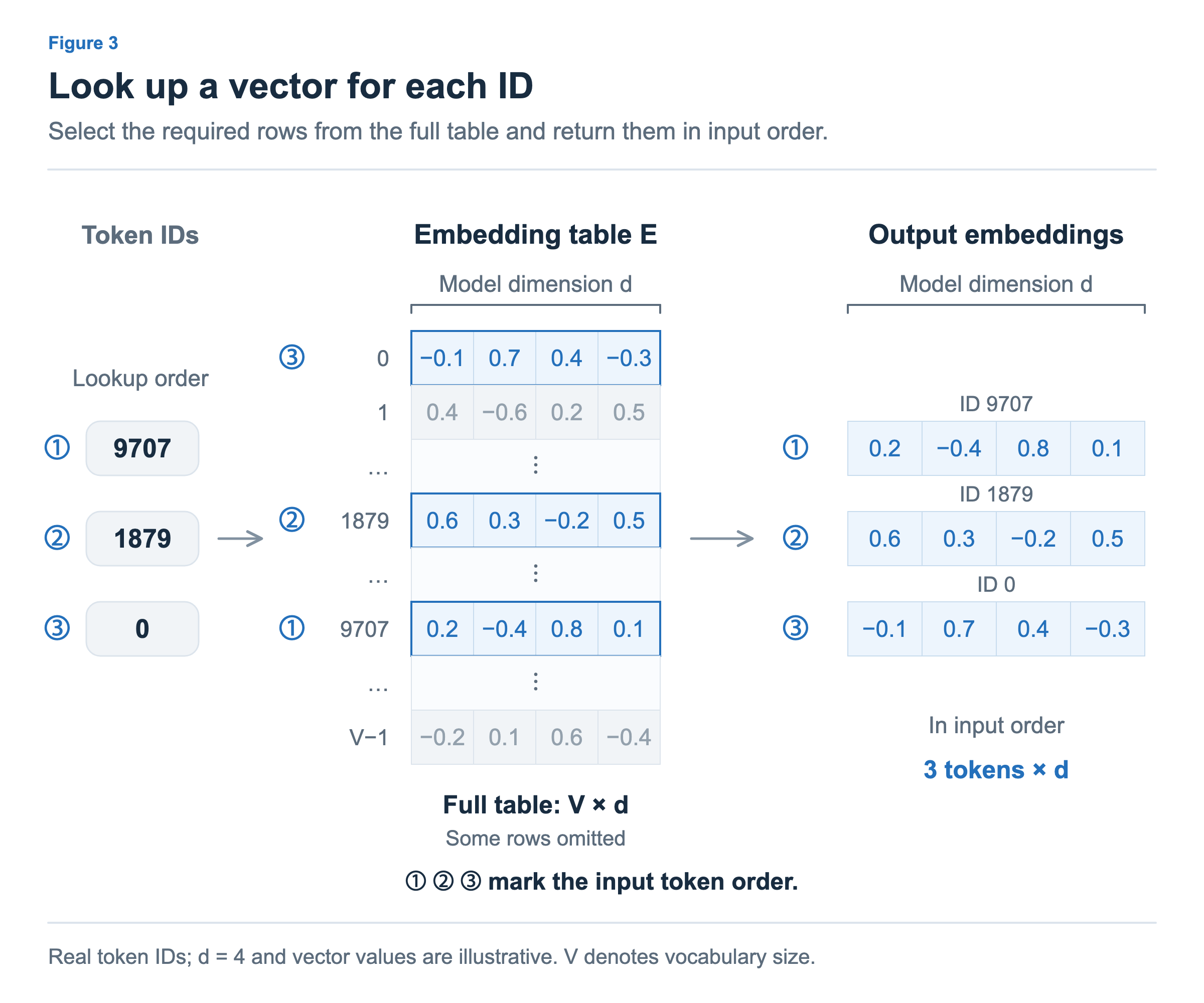
For an input ID of 9707, the layer retrieves the corresponding row of the table. Three input token IDs produce three vectors in the same order. This operation is called an embedding lookup. The diagram omits some rows of the full table and highlights the three rows being looked up. Regardless of their row order in the table, the output follows the input ID order: 9707, 1879, 0. The four-dimensional vectors and their values are illustrative examples.

Decoder Blocks: Dimensions Stay the Same, Vector Values Change

The vectors from the embedding layer enter a decoder block. If there are T tokens and each vector has dimension d, we can represent the input as a T × d array with T rows and d columns. Each row represents one token. The decoder block performs computations on these representations and returns an output with the same T × d shape. The diagram omits the batch axis to focus on a single input sequence.

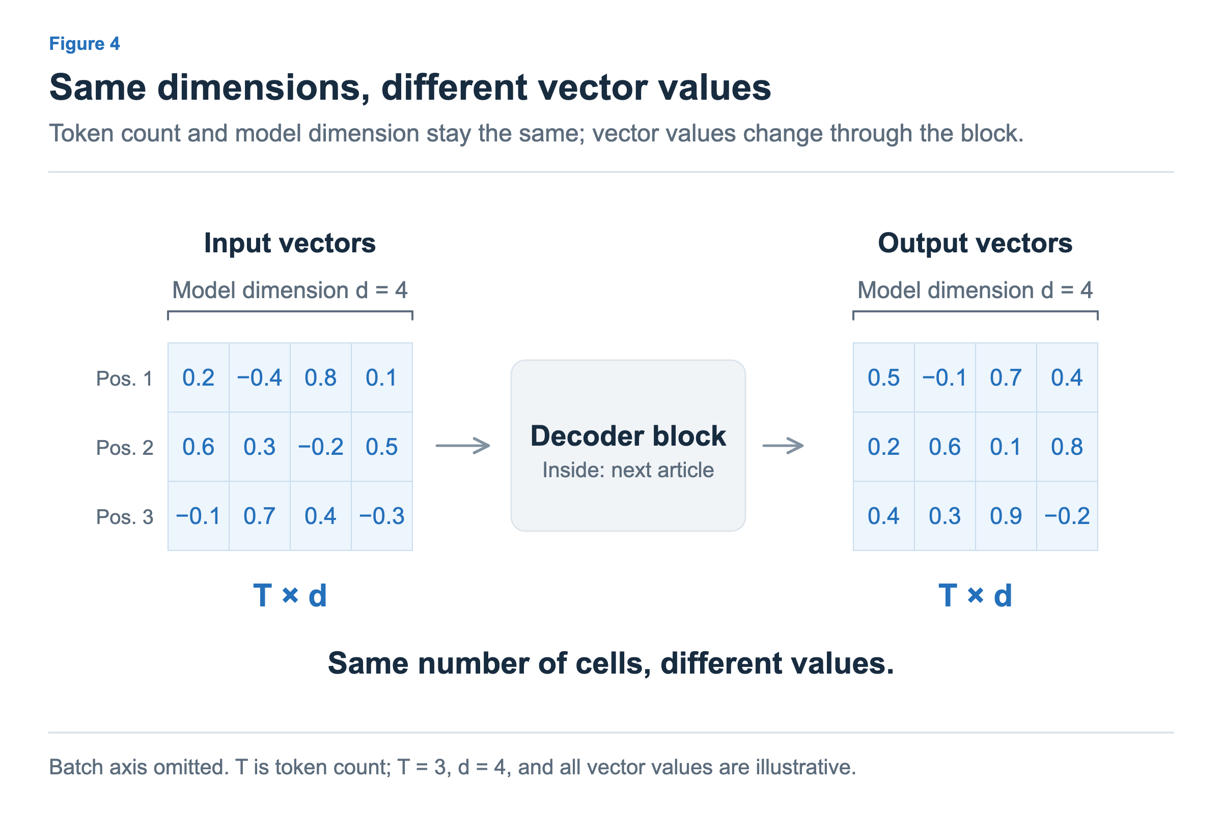
The important point is that the vector values change even though the input and output dimensions are the same. As tokens pass through a decoder block, their vector values change to incorporate information from preceding tokens. The output then becomes the input to the next decoder block. Multiple blocks transform the vector values in sequence while maintaining the same input and output shape. Starting with the next article, we will examine the internal structure responsible for these transformations.

The LM Head: Converting Vectors to Vocabulary Scores

After passing through the decoder blocks and the final normalization, the token representations enter the LM Head. Through matrix multiplication with learned weights, the LM Head maps each token’s d-dimensional representation to V scores. V is the vocabulary size, and each output score corresponds to one token in that vocabulary. The overall shape therefore changes from T × d to T × V. Rows still correspond to token positions, while columns change from model features to vocabulary scores.

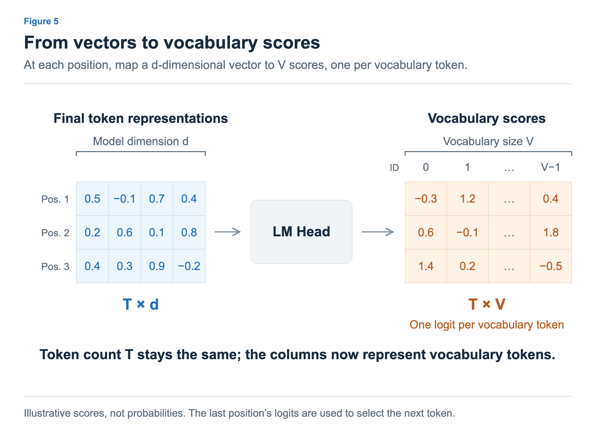
These scores are called logits. Logits are not yet probabilities; they provide the basis for selecting the next token. During generation, we use the scores from the last input position. For example, with three input tokens, the scores at the third position are used to select the following token. The embedding layer retrieves vectors for input IDs, while the LM Head uses vectors that incorporate context to calculate scores for possible next tokens.

We have now followed the full path from text to token IDs, vectors, and vocabulary scores. In the next article, we will examine the internals of the decoder block that we have represented as a single box. We will begin with residual connections and RMSNorm to understand the block’s structure and see where Attention and the MLP fit within it.