Reducing Memory Traffic with Output Accumulation in FlashAttention

The previous article introduced online softmax, which updates the maximum and exponential sum while reading scores in chunks. Computing these two values, however, does not output the probabilities at every position. Attention needs the final output: a weighted sum of Value vectors using those probabilities. If we can accumulate this output with each chunk of scores, we can continue computing without storing large score and probability matrices.

We will first explore why we can compute the Value weighted sum and divide by the exponential sum at the end. Then we will see how to rescale and add to the exponential sum and weighted sum using the same reference as new scores arrive. We will apply this rule to small Q, K, and V tiles, follow the output to completion, and examine how this reduces the storage and rereading of large intermediate matrices. Connecting a mathematical accumulation rule to actual savings in data movement is central to FlashAttention.

The specific computation order in this article follows the FlashAttention-2 forward algorithm. Accumulating outputs tile by tile to avoid storing large intermediate matrices was already part of the original FlashAttention. Normalizing just once after processing all tiles is a FlashAttention-2 improvement.

Computing the Value Weighted Sum First

Basic attention computes scores from Q and K, turns them into probabilities with softmax, and then uses those probabilities as weights to sum V. For one query, there is one score for each key, and each score corresponds to the Value vector of the same token. Keys help determine how much to include; Values hold the content included in the output.

Stable softmax subtracts the same maximum m from every score before applying exp. The sum of these exponentials is ℓ, and dividing each exponential by ℓ gives a probability. All probabilities for one query share the denominator ℓ, so instead of dividing each weight before summing the Values, we can compute the weighted sum first and divide once at the end. Here, dividing once means dividing every element of the output vector by the same ℓ.

In Figure 1, the scores are [1, 2], and their Values are [2, 0] and [0, 2]. Subtracting the maximum 2 gives exponentials of about [0.368, 1] and an exponential sum of about 1.368. Computing the probabilities first gives about [0.269, 0.731], so the output is 0.269 × [2, 0] + 0.731 × [0, 2] ≈ [0.538, 1.462]. Decimals in this article and its figures are rounded after calculation at full precision.

Deferring division lets us weight the Values directly with the exponentials. We compute 0.368 × [2, 0] + 1 × [0, 2] ≈ [0.736, 2], then divide this vector by the exponential sum of about 1.368 to obtain the same output [0.538, 1.462].

Let a denote this Value weighted sum before division by the exponential sum. It is a vector with the same length as a Value, rather than a single scalar. From here on, we accumulate both the sum of exponentials ℓ and the exponential-weighted Value sum a. Once all scores have been included, O = a ÷ ℓ gives the final output O.

Updating the Exponential Sum and Weighted Sum Together

Processing scores in chunks means the maximum m can change along the way. Just as we rescaled the previous exponential sum to a new maximum, we must also rescale the previous weighted sum a to the same reference. When m increases, all previous exponentials are multiplied by the same factor. The V multiplied by each exponential stays unchanged, so we can multiply the entire accumulated sum a by that factor as well.

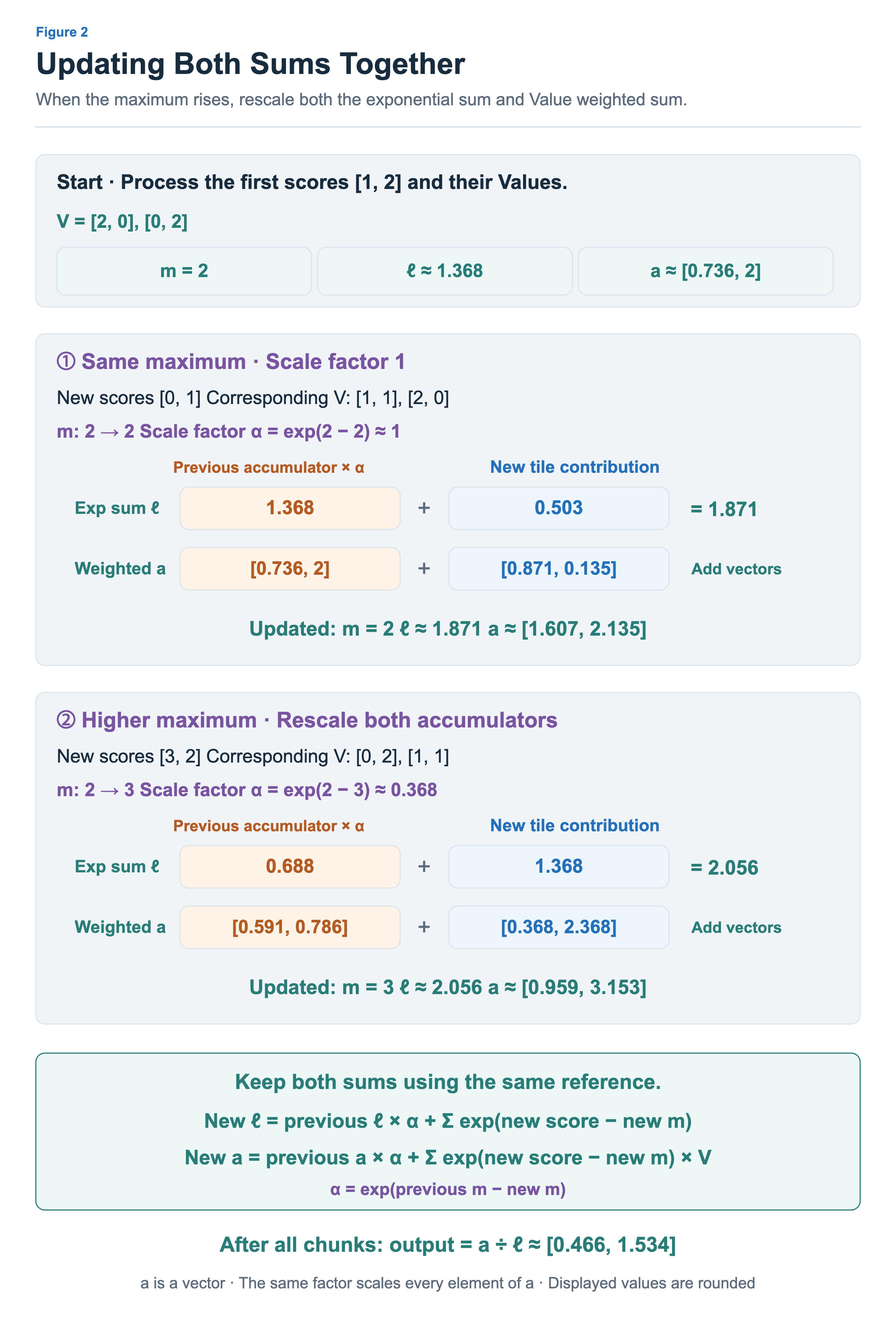
Figure 2 processes the scores [1, 2, 0, 1, 3, 2] for one query two at a time. After processing the first chunk [1, 2] with Values [2, 0] and [0, 2], we have m = 2, ℓ ≈ 1.368, and a ≈ [0.736, 2]. We keep these three state values and read the next chunk.

Adding New Contributions When the Maximum Stays Unchanged

The second score chunk is [0, 1], with Values [1, 1] and [2, 0]. Both scores are below the previous maximum 2, so m stays at 2. The previous ℓ and a already use this reference and can be kept as they are.

The new exponentials are about [0.135, 0.368]. We add their sum, about 0.503, to ℓ. To the weighted sum, we add 0.135 × [1, 1] + 0.368 × [2, 0] ≈ [0.871, 0.135]. After two chunks, we have ℓ ≈ 1.871 and a ≈ [1.607, 2.135].

Rescaling Both Accumulators When the Maximum Increases

The third chunk [3, 2] introduces a larger score, 3. Changing m from 2 to 3 requires multiplying all previous exponentials by exp(2 − 3) ≈ 0.368. We can multiply the accumulated ℓ and a by this factor without rereading previous scores or Values.

The previous exponential sum of about 1.871 rescales to about 0.688. The previous weighted sum [1.607, 2.135] rescales to about [0.591, 0.786]. The same factor applies to every element of the weighted-sum vector.

We now compute exponentials for the new scores [3, 2] using the new maximum 3. They are about [1, 0.368], with Values [0, 2] and [1, 1]. Adding the new exponential sum of about 1.368 and weighted sum of about [0.368, 2.368] gives ℓ ≈ 2.056 and a ≈ [0.959, 3.153]. With all scores processed, dividing a by ℓ yields an output of about [0.466, 1.534].

The rule is the same in both cases. Choose the new maximum, rescale the previous exponential sum and weighted sum by the same factor, and add the contributions from the new scores and Values. If the maximum stays unchanged, the factor is simply 1. We can maintain the information needed for the final output without completing the final probabilities in each tile. Algorithm 1 in FlashAttention-1 maintains a partial output O divided by the new exponential sum after every tile. At the next tile, it multiplies by the previous exponential sum to recover and rescale the weighted sum before adding the new contribution. In contrast, Section 3.1.1 and Algorithm 1 in FlashAttention-2 maintain the unnormalized weighted sum a and divide just once at the end, reducing repeated normalization. Both versions already weight V with exponentials.

Completing the Output by Traversing Tiles

So far, we have paired Values with scores that were already given. Actual attention multiplies Q and K to form a score tile, then continues directly with exponentials and the Value weighted sum. A tile is a small matrix region processed together. Keeping one Q tile while reading K and V in matching token ranges lets us apply the same accumulation rule.

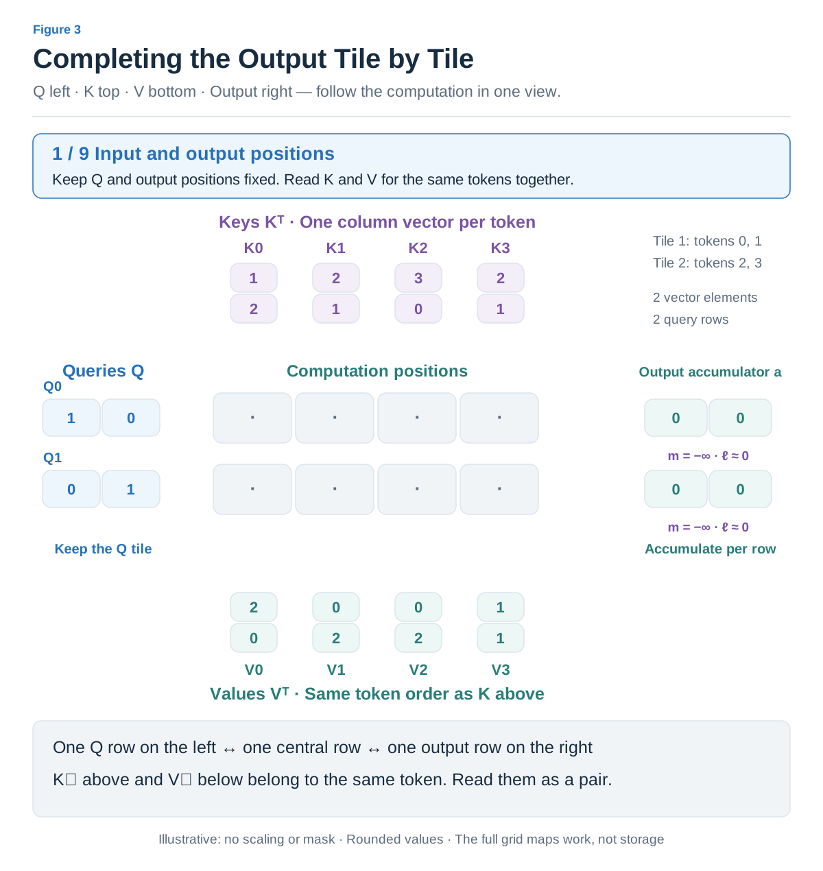
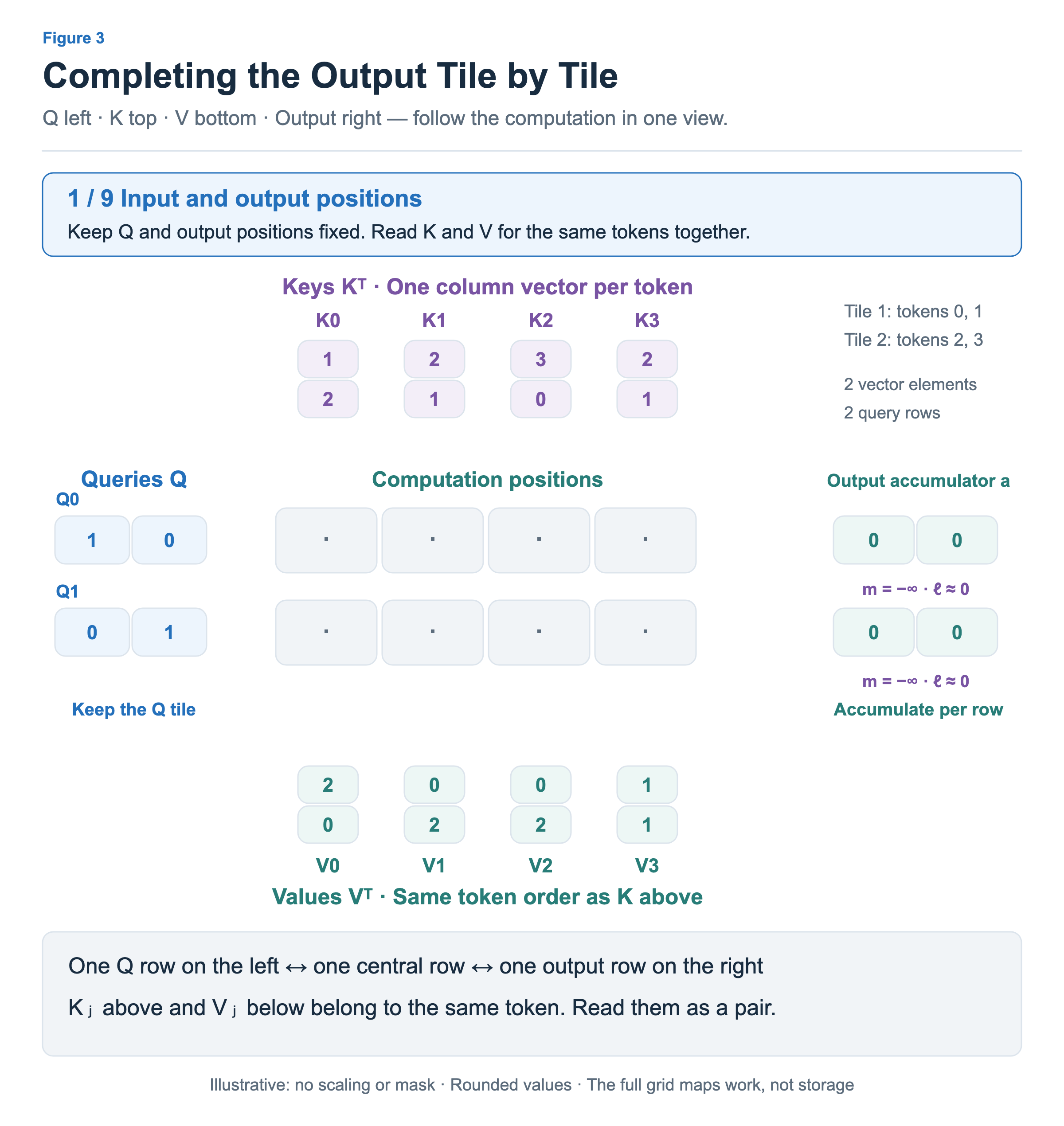
Figure 3 places two queries on the left, four keys at the top, four Values at the bottom, and output accumulators on the right. Each Q row on the left corresponds to an output row on the right. K at the top and V at the bottom are vertically aligned by token. To align token positions, the figure lays out K and V as Kᵀ and Vᵀ, but the actual Value weighted sum multiplies the exponential-weight tile by the V tile.

Use “Next” below to follow the steps. This small example omits scaling and masking to make the numbers easy to follow. Standard attention divides the Q–K dot product by the square root of the key-vector dimension d and applies a mask when needed. These operations happen before exp, and the accumulation rule that follows stays the same.

View Figure 3 step by step on a separate page

Keeping Q While Processing the First K/V Tile

The first tile reads K₀, K₁ and V₀, V₁. Since Q₀ is [1, 0] and K₀ is [1, 2], their dot product is 1 × 1 + 0 × 2 = 1. Computing the dot products for the two queries and two keys produces a 2 × 2 score tile in the center. Q₀ has scores [1, 2], and Q₁ has scores [2, 1].

Subtracting each row’s maximum and applying exp gives about [0.368, 1] for Q₀ and [1, 0.368] for Q₁. Both rows have a maximum of 2 and an exponential sum of about 1.368. The central exponentials are not yet final probabilities. Scores from keys read later must also contribute to the exponential sum.

We can nevertheless weight the Values with these exponentials immediately. V₀ is [2, 0] and V₁ is [0, 2], so the first tile’s weighted sum is about [0.736, 2] for Q₀ and [2, 0.736] for Q₁. We keep these vectors on the right. Even when processing multiple queries together, each query row has its own maximum, exponential sum, and weighted sum.

Moving K/V and Accumulating into the Same Output

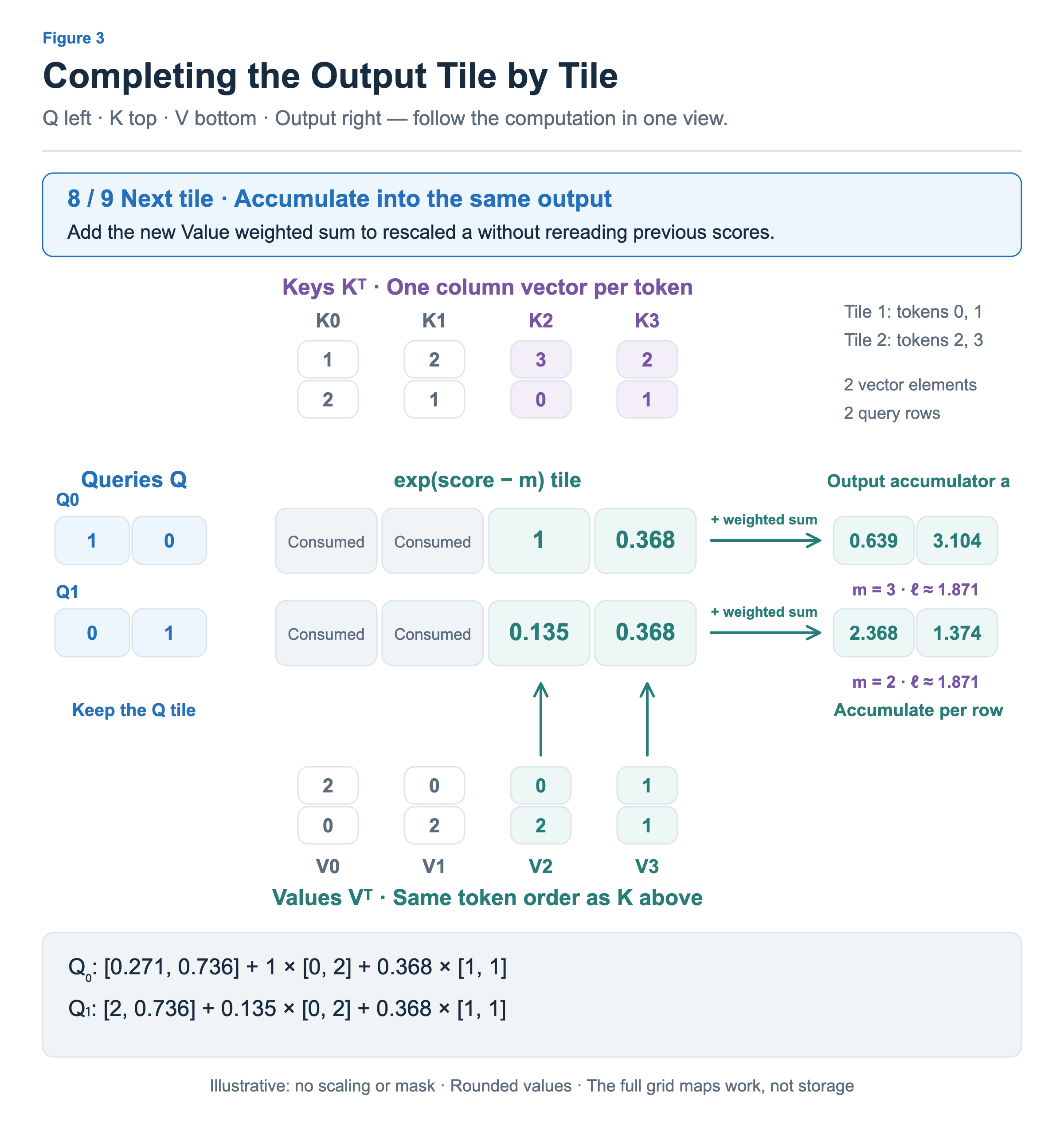
Next, the highlighted regions at the top and bottom move together to K₂, K₃ and V₂, V₃. Q on the left and the accumulators on the right stay in place. Computing the new score tile with the same Q gives [3, 2] for Q₀ and [0, 1] for Q₁.

Q₀’s maximum rises from 2 to 3, so we multiply its previous ℓ and a by about 0.368. Q₁ keeps its previous maximum 2, so its scale factor is 1. We then add the sum of the new exponentials to each ℓ and the new Value weighted sum to each a, using the new reference. Different rows can need different rescaling within the same tile.

The central cells of the first tile now read “Consumed.” Their scores and exponentials have already contributed to the exponential sum and weighted sum, so they need not be kept to continue this forward computation. The full central grid is a map of computation positions, not storage for the full score matrix.

Normalizing After All Tiles Have Contributed

After both tiles, the final exponential sum is about 1.871 for each row. The weighted sums are about [0.639, 3.104] for Q₀ and [2.368, 1.374] for Q₁. Dividing each by its row’s exponential sum gives final outputs of about [0.341, 1.659] for Q₀ and [1.266, 0.734] for Q₁.

The two matrix multiplications in this process are clear. First, the Q and K tiles compute scores. Then the exponential-weight tile and V tile compute vectors to add to the output. Online softmax rescaling and updates connect them. Like the Q tile in the figure, other Q tiles can maintain their own outputs and state while processing the required K/V tiles.

Reducing the Storage and Rereading of Intermediate Matrices

This computation order matters because it changes which data moves within the GPU. Basic attention in Figure 4 stores a large score matrix S in global memory and reads it again for softmax. It also stores the resulting large probability matrix P and reads it again to multiply by V. For sequence length N, each head’s score and probability matrices are each N × N, so the intermediate-data burden grows rapidly with sequence length.

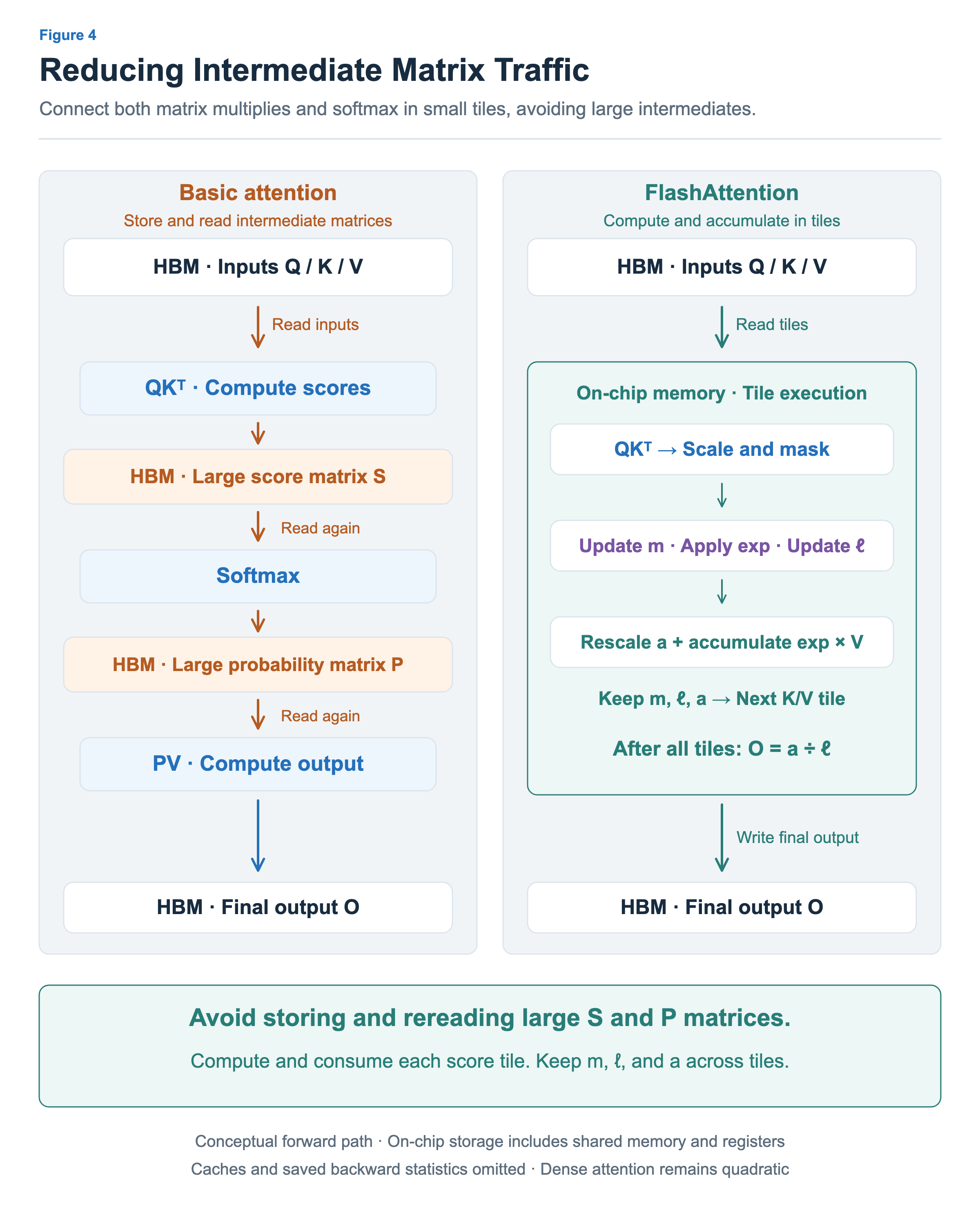
FlashAttention computes the current score tile and immediately uses it for exponentials and the Value weighted sum. It keeps the Q tile and accumulation state on chip while reading the next K/V tile, then writes the final output after all tiles have contributed. Here, on-chip memory refers to shared memory, registers, and other storage close to computation. This avoids storing the entire large S and P matrices in global memory and rereading them in subsequent stages. FlashAttention’s memory-traffic optimization

The figure simplifies the main flow between HBM and on-chip memory. Caches participate in actual global-memory accesses, so not every access is equivalent to an HBM transfer. The figure also omits operations such as saving per-row normalization statistics for the backward pass during training. The distinction to focus on is storing large N × N intermediate matrices versus computing and consuming small tiles.

The optimizations introduced earlier come together here. Tiling divides inputs into small regions that can be loaded and reused. Fusion reduces intermediate data movement between score computation, softmax, and the Value weighted sum. Online updates make it possible to complete the output even when softmax, which needs the entire row, is split across small tiles. Online accumulation is what connects tiling and fusion across the full attention computation.

FlashAttention does not turn the quadratic operation count of standard dense attention into a linear one. Its key benefit is reducing data movement and intermediate storage without switching to approximate attention, although actual floating-point results can differ due to computation order. This article focused on the forward-pass principle. Version-specific thread layouts, pipelines, and backward recomputation are separate optimizations built on this principle.