From Operation Optimization to Whole-Model Performance

In the previous article, we explored how FlashAttention reduces the storage and rereading of large score and probability matrices. But a model does more than compute attention. Even after attention becomes faster, other operations such as the MLP and normalization still need to run. The benefit of speeding up one operation must be checked in the execution time of the whole model.

This article uses a small example to show how much improving one part reduces the total time. We then explore why the main bottleneck can change during optimization, leading us to repeat improvements and measurements. Finally, we move beyond using the current GPU’s resources efficiently to consider using more resources according to execution goals and memory capacity.

Improving One Operation and the Total Execution Time

Suppose it takes 100ms to compute a model’s output once for a fixed input. Here, the full execution means one forward pass. This measurement covers a different scope from a service’s response time, which may include repeated token generation or time spent waiting in a request queue.

Assume that attention takes 60ms of those 100ms, the MLP takes 30ms, and the rest takes 10ms. Attention in this example means the core attention portion to which FlashAttention applies; QKV and output projections, normalization, and other operations are included in the rest. These numbers are assumptions used to explain the principle, not the time breakdown of a particular model or actual FlashAttention measurements.

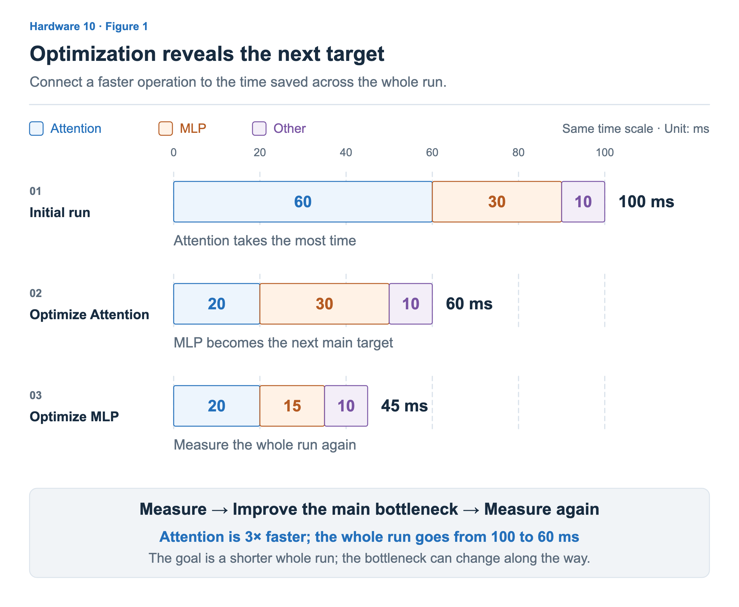
Figure 1 groups the time spent across multiple layers by operation type. It does not mean that the actual model runs all attention operations before all MLP operations. This example also assumes that operations do not overlap, so adding the times of the individual parts gives the total time.

First, we improve attention and reduce its time from 60ms to 20ms. Looking at attention alone, 60 ÷ 20 = 3, so it runs three times as fast. But the MLP’s 30ms and the other operations’ 10ms remain unchanged. The total time becomes 20 + 30 + 10 = 60ms, a reduction of 40ms from the original. Attention is three times as fast, but the whole model is only about 1.67 times as fast.

Even if we reduce attention time to almost zero in this example, the 40ms needed for the MLP and other operations remains. No matter how fast attention becomes, improving it alone cannot bring the total execution time below 40ms. The central idea of Amdahl’s law is that the time spent in the parts we do not improve sets a limit on the overall speedup. When considering a new optimization technique, we should also check how much of our execution time is spent in the part it speeds up.

Bottlenecks Change During Optimization

In the first stage of Figure 1, attention accounts for the most time at 60ms. After we reduce it to 20ms, the MLP’s 30ms becomes the largest part. The MLP itself has not become slower. As attention time decreases, the MLP’s share of total execution grows from 30% to 50%.

We can now examine the MLP’s execution and look for improvements in input reuse or data movement. If we reduce the MLP from 30ms to 15ms as in the example, the total becomes 20 + 15 + 10 = 45ms. Attention is once again the largest part at 20ms. A part we optimized earlier can become an important target again after we improve other parts.

Earlier articles explored why an operation can be limited by the rate at which it fetches data from memory or the rate at which the compute units process it. We now extend that observation to the whole model. We identify the parts that account for much of the total time, then examine which resources limit execution within those parts. If we find that the MLP takes a large amount of time, we must choose how to improve it by looking at matrix shapes, data reuse, and compute utilization.

This process repeats as measure → improve the main bottleneck → measure again. The goal is to reduce total execution time; a change in the bottleneck is one possible result of that process. The same part may still account for the largest share after an improvement. A part with a large time share may also have little room for improvement if it already runs efficiently, so we need to consider both its share and its potential for improvement. The CUDA optimization guide also emphasizes this iterative approach.

When comparing execution before and after an improvement, we should measure the same scope using the same model, input size, data type, and device. We distinguish the time of a particular kernel from the time of the whole model, and consistently decide whether to include first-run setup costs. GPU work can execute asynchronously, so the time the CPU takes to submit work must not be interpreted as the time the GPU takes to finish computing. GPU timing must use the start and completion of the work being measured as its reference points.

Although we added the times of the individual parts in Figure 1, actual execution may fetch data for the next computation while the current computation is running. Adding compute time and data movement time directly would then count the time spent running simultaneously twice. We must therefore check not only the time of each part, but also the time from starting model execution until all the required work finishes.

The main bottleneck can also change when the input changes. For example, unlike processing a single token in a matrix multiplication, processing multiple tokens together lets us reuse the fetched weights across those tokens’ computations. This can reduce the cost of reading weights per token, changing the time shares of computation and data movement. To find out whether an optimization that worked well for one input is also effective for another, we must run it again with that input.

Adding Resources to Meet the Goal

So far, we have looked at reducing unnecessary data movement and waiting, and making better use of the compute units on a given GPU. These improvements matter for getting better performance from the same resources. But depending on the capacity required for execution and the performance goals we want to meet, using more resources may also be necessary.

Execution Time and Throughput Goals

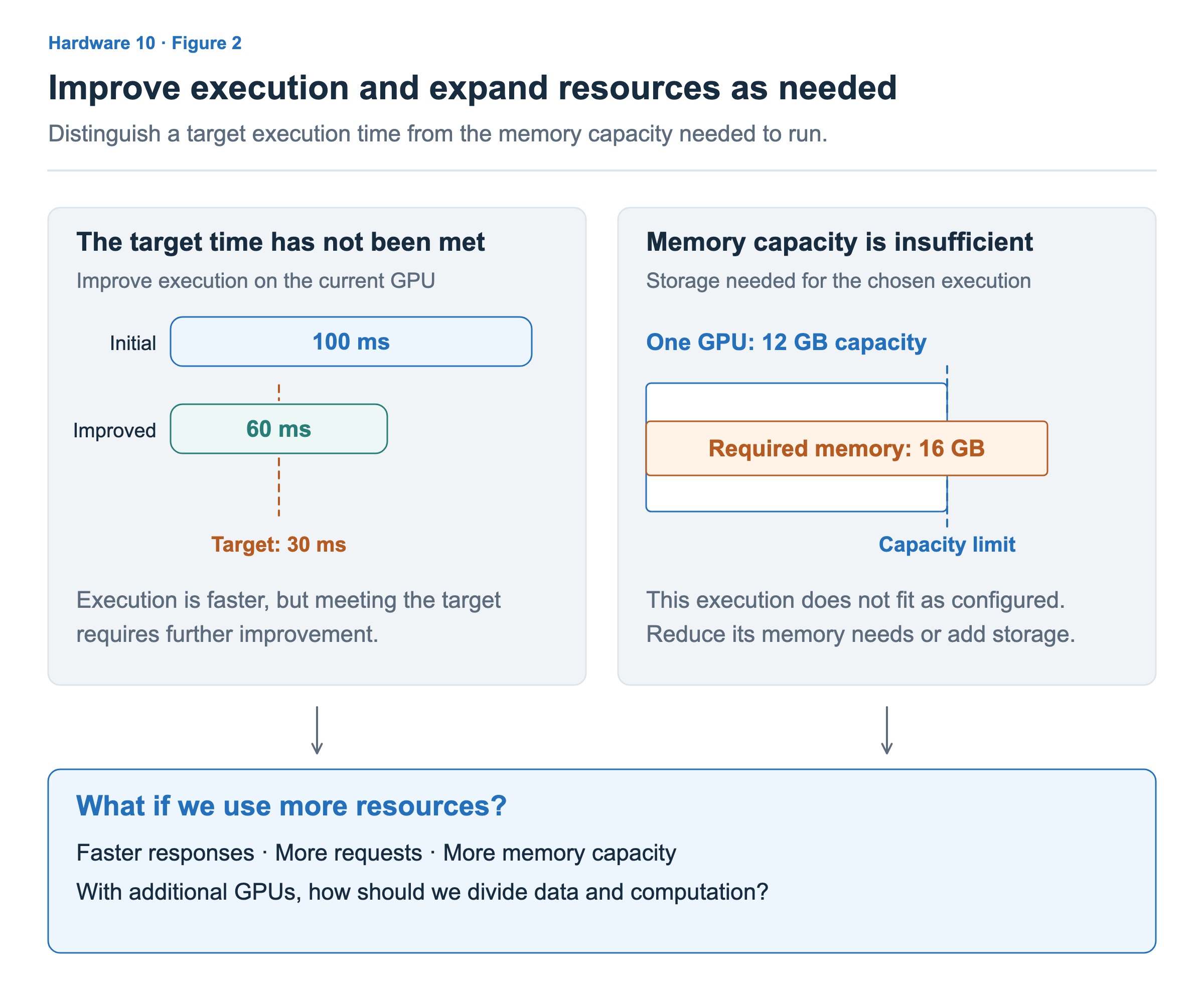
On the left of Figure 2, we have reduced execution time from 100ms to 60ms but have not reached the target of 30ms. We could make further improvements on the same GPU, or consider dividing computation across multiple GPUs to reduce completion time. Here, 30ms is an illustrative target; the appropriate performance goal depends on the requirements of the actual workload.

Apart from how long one task takes to finish, the number of tasks that must be processed in the same amount of time may increase. Even if each request is processed fast enough, more incoming requests require resources to process more of them together. If the model fits on one GPU, we can consider placing the same model on multiple GPUs and assigning different requests to each. This is why we distinguish reducing the time of one request from increasing the throughput of the entire service.

Memory Capacity Needed for Execution

The right side of Figure 2 shows a case where capacity is a problem before speed becomes the issue. If one GPU has 12GB of memory but the chosen execution requires 16GB, that GPU cannot hold all of the required state. The requirement includes not just weights but also intermediate values and other state that must be held at the same point during execution.

We can reduce the requirement by avoiding unnecessary intermediate storage, as FlashAttention does. But if such improvements still cannot fit the chosen model and input into the available memory, we need to change the execution conditions or increase the available storage resources. Distributing the model and required state across multiple GPUs is one option to consider. Reading data quickly and having enough space to hold the required data are different problems.

We can consider optimizing current resources and adding resources together. We do not need to finish every possible improvement on one GPU before using multiple GPUs. The choice depends on whether memory capacity is insufficient, one request takes too long, or more requests must be processed in the same amount of time.

Adding GPUs provides more compute units and memory. To use those resources, we must decide which data and computation each GPU should handle and transfer the data they need from one another. In the next article, we will explore what using multiple GPUs means, the benefits of the added resources, and the communication and waiting that we need to consider.