Scaling Across Multiple GPUs

In the previous article, we explored the process of improving one operation, measuring the whole model again, and finding the next bottleneck. Alongside using the same GPU more efficiently, we could also consider adding resources according to memory requirements and performance goals.

Adding GPUs provides more compute units and memory. But using those added resources requires deciding where to place data and computation. So far, we have examined execution time mainly through memory traffic and computation within one GPU. When we divide computation across multiple GPUs, we also need to consider the time spent exchanging required data and waiting for another GPU’s results to become ready. Alongside memory traffic and computation within each GPU, communication and waiting between GPUs also affect overall performance.

This article first examines how compute units and memory are divided across multiple GPUs. We then distinguish running a larger model, finishing one request faster, and processing more requests. Finally, we explore the communication and waiting that connect divided computation, and why speed does not increase in proportion to the number of GPUs.

Each GPU’s Compute Units and Memory

So far, we have looked at fetching data from memory, computing, and storing results within one GPU. When we use two GPUs, each has its own compute units and memory. We need to distinguish data stored on GPU 0 from data stored on GPU 1 and check where the inputs required for each GPU’s computation reside.

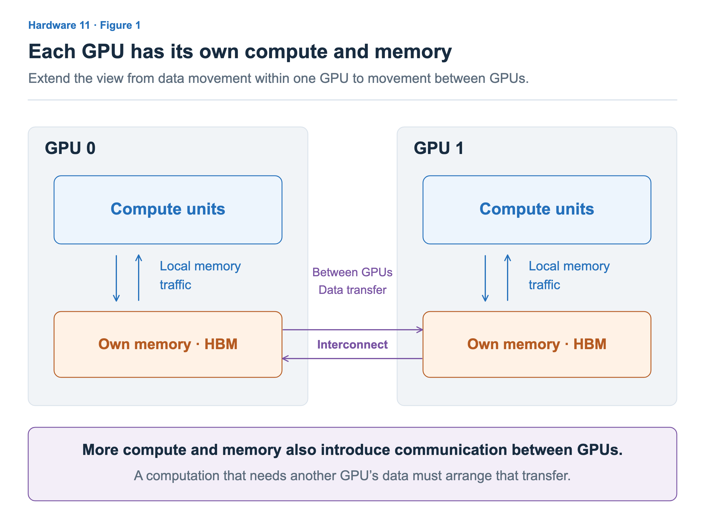
In Figure 1, the blue arrows show the familiar movement of data within a GPU. The purple arrows show the path for exchanging data with another GPU. If GPU 1’s next computation needs a result produced by GPU 0, that result must be transferred so GPU 1 can use it. Communication is also data movement; here, its scope extends across GPUs.

Having more memory capacity across two GPUs does not automatically make an existing execution use one large memory. The execution software must manage which data is stored on which GPU and when to transfer data needed by another GPU. To show this relationship, the figure groups memory and compute units broadly, omitting the caches, shared memory, and registers within each GPU.

The paths connecting GPUs are also part of the execution conditions. GPUs within the same server and GPUs in different servers may use different communication paths. For example, NVIDIA’s GPU communication library, NCCL, supports several connection types, including PCIe, NVLink, and networks between servers. Before considering specific communication methods, we start by looking at where the data to be computed is located and which path it will travel.

Three Reasons to Use Multiple GPUs

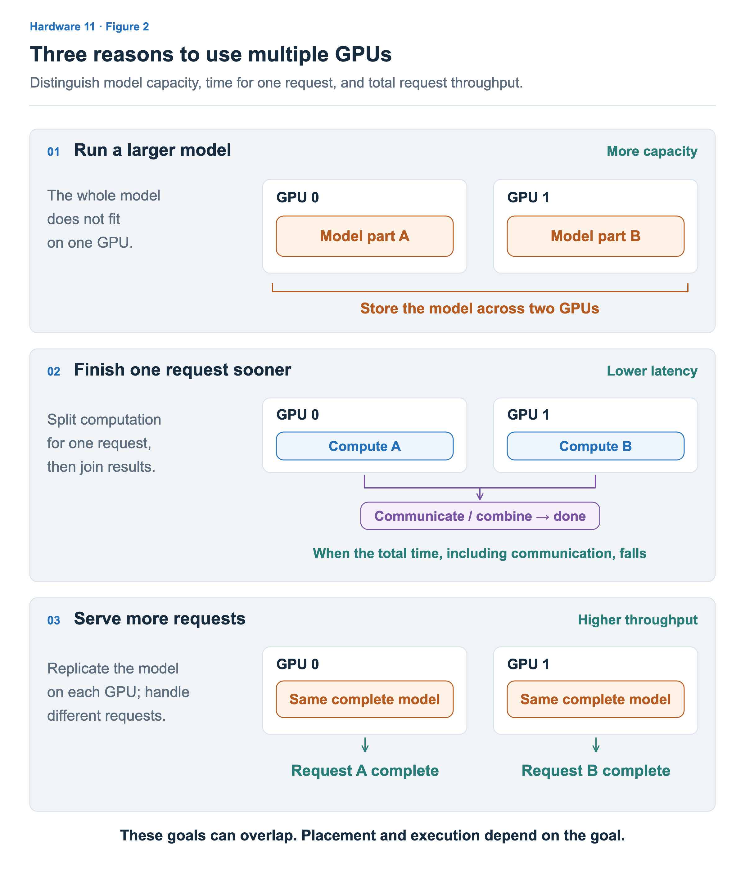
The data we place and the computation we divide depend on why we are adding GPUs. Figure 2 distinguishes the intended benefit even when using the same two GPUs.

Running a Larger Model

If it is difficult to store the whole model on one GPU, we can distribute it across multiple GPUs. In the first panel of Figure 2, part A of the model is stored on GPU 0 and part B on GPU 1. Each GPU also needs intermediate values and workspace for its assigned computation, so we must check memory usage during execution as well as the size of the weights.

The intended benefit here is the capacity to run a model that was difficult to fit on one GPU. Dividing storage alone does not mean that computation proceeds simultaneously or that one request becomes faster. If B requires A’s result before it can be computed, data must be transferred and computation executed according to that dependency.

Finishing One Request Faster

To reduce the time until one request finishes, we divide the parts of its computation that can run together. In the second panel, GPU 0 and GPU 1 perform computations A and B, then combine their results to finish the request.

Even if each GPU has less computation to do, time may be added to distribute inputs or collect results. To finish the request faster, the time saved in computation must exceed the added communication and waiting. What can be divided and which results must be collected depend on the original operation’s dependencies.

Processing More Requests

If the model fits on one GPU, we can place the same model on each GPU and assign different requests, as in the third panel. GPU 0 processes request A, and GPU 1 processes request B. Unlike dividing one request’s computation in two, each GPU performs the model computation needed for its own request.

The goal here is to increase the number of requests completed in the same amount of time. Even if each request’s compute time stays the same, two GPUs can increase overall throughput by processing different requests together. This approach does not require collecting intermediate results within one request across GPUs, but we still need to decide which GPU handles each request.

These three purposes can also occur together. For example, we can run one model across multiple GPUs and create several such GPU groups to process different requests. Distinguishing the required capacity, response time, and throughput goals first makes it easier to decide what placement is needed.

Communication Connects Divided Computation

After dividing the model and computation, we must check what form of input the next computation requires. Having results on individual GPUs does not by itself let the model’s next step execute immediately.

For example, if two GPUs each finish one part of an output vector, the next computation may require a vector assembled from those pieces. In contrast, if we split the products within a single dot product into two groups, each GPU obtains a partial sum contributing to the same output value. We must add the two values to obtain the final output. Joining pieces and adding partial sums for the same positions are different operations.

The transfer method also depends on whether only one GPU will use the final result or several GPUs will all use it. Communication operations that handle these differences include gathering data and adding partial results before distributing them. NCCL’s communication operations also distinguish the meanings of these data exchanges. We will explore the names and specific flows of each operation in the next article.

The placement of data and computation also affects communication volume. A placement that can use a result directly in the next computation requires different transfers from one that must fetch another GPU’s results each time. We should therefore decide where to divide computation together with where to exchange data. Communication includes not only the time to move data, but also the cost of starting communication and coordinating the readiness of participating GPUs, so we need to consider both the amount of data exchanged and the number of exchanges.

Execution Time with Communication and Waiting

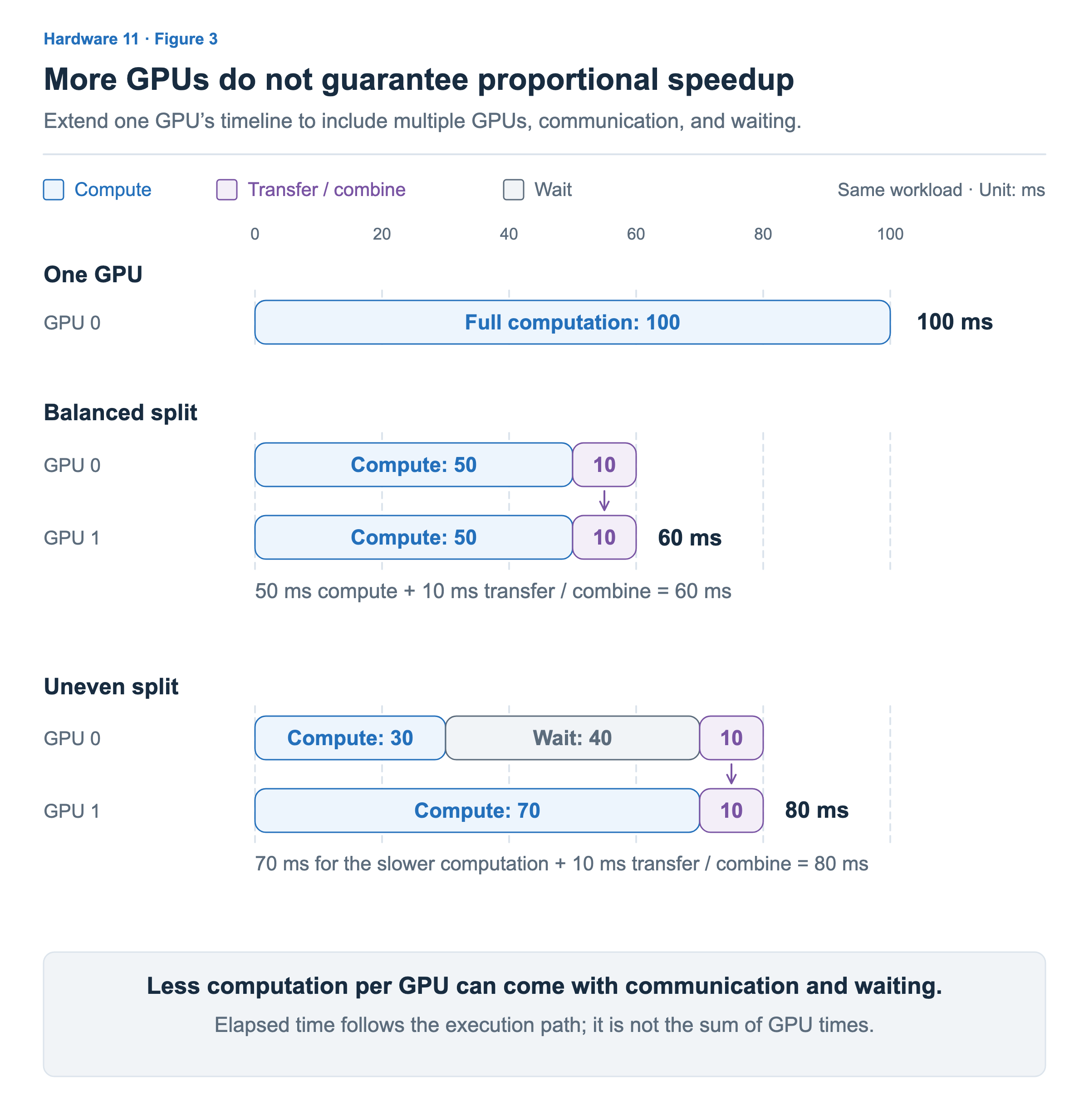
How does dividing computation change the actual completion time? Figure 3 shows an example of splitting the same task that took 100ms on one GPU across two GPUs. The numbers are illustrative. We assume that each GPU computes at the same speed and that communication and result combination follow computation. Computation and communication do not overlap in this example.

When Computation Is Split Evenly

In the middle of Figure 3, the two GPUs each perform 50ms of computation simultaneously. Computation alone has been reduced from 100ms to 50ms. But transferring and combining results adds 10ms, so the total completion time is 50 + 10 = 60ms. Even with two GPUs, the overall speedup is 100 ÷ 60 ≈ 1.67 times.

The purple 10ms intervals in the two GPU rows represent time spent participating in the same communication and combination. One GPU’s 10ms does not follow the other GPU’s 10ms. Instead of adding the times of individual GPUs, we must look at when computation and transfer finish on the same time axis.

When More Computation Falls on One GPU

At the bottom of Figure 3, GPU 0 is assigned 30ms of computation and GPU 1 is assigned 70ms. GPU 0 finishes computing first, but GPU 1’s result, which is needed for the next step, is not ready yet. GPU 0 therefore waits 40ms before joining the communication and combination. Checking that the work required for the next step has finished and coordinating the order in which work proceeds is synchronization. If another GPU’s computation or data transfer has not finished yet, synchronization can involve waiting.

The whole task finishes in 80ms: the slower computation’s 70ms plus 10ms for communication and combination. GPU 0’s 40ms wait overlaps with GPU 1’s computation. We therefore do not add that waiting time to the 80ms again. Even if one GPU finishes early, overall completion is delayed when the next step must wait for another GPU’s result.

To reduce this wait, we should examine whether the work can be divided more evenly or whether another task that does not depend on the awaited result can be performed. The same applies to communication. Once the required data is ready, there may be room to start communication and run computation that does not yet need its result alongside it. However, computation that requires the transfer to finish must wait for its completion.

With multiple GPUs, we consider computation, memory traffic within each GPU, and communication between GPUs together. We do not always add these three times separately; we check what proceeds concurrently and what makes the next task wait. Communication may also share resources with internal memory accesses, so the effect of overlapping execution must likewise be judged by the overall completion time.

Just as we checked the overall bottleneck again after improving one part in the previous article, observation continues after adding GPUs. Communication may account for a larger share as compute time decreases, or work concentrated on a particular GPU may become the next target for improvement. The next article will examine basic communication methods for sending and gathering data between GPUs, following which data each GPU starts with and which results it obtains in detail.