KV Cache Management and PagedAttention

Batching and Scheduling showed that a new request may have to wait even when there is enough capacity to hold the actual KV. If an ongoing request reserves a large region for its future growth, even the empty part cannot be given to another request.

To reduce this problem, the engine must be able to allocate space as KV grows. To avoid moving existing data into a larger region each time, it must also be able to compute with a request’s KV stored in separate locations.

This article begins with allocating KV storage in small blocks and connecting token order to actual storage locations. It then explains how PagedAttention reads scattered KV, followed by how sharing common KV reduces storage when generating multiple responses from the same input.

Allocate blocks as needed

We will continue with B and C from the previous article. Excluding weights and computation workspace, the KV capacity holds 24 token positions. B currently has KV for 6 positions but has reserved space for 20 to allow for future generation. Only 4 positions remain available for a new request, so C, with 6 input tokens, cannot join.

Now let us divide that space into smaller units. A block is a fixed-size storage unit that holds KV for several token positions. In this example, one block stores KV for four positions. The 24 slots therefore correspond to 6 blocks. A cell in the figure represents space for the K and V computed at that position, not the token itself.

B needs 2 blocks to hold its current KV for 6 positions. Allocating 8 slots leaves 6 occupied and 2 empty. B still fits when processing its next input increases its stored KV to 7 positions. C’s 6 input tokens also need 2 blocks.

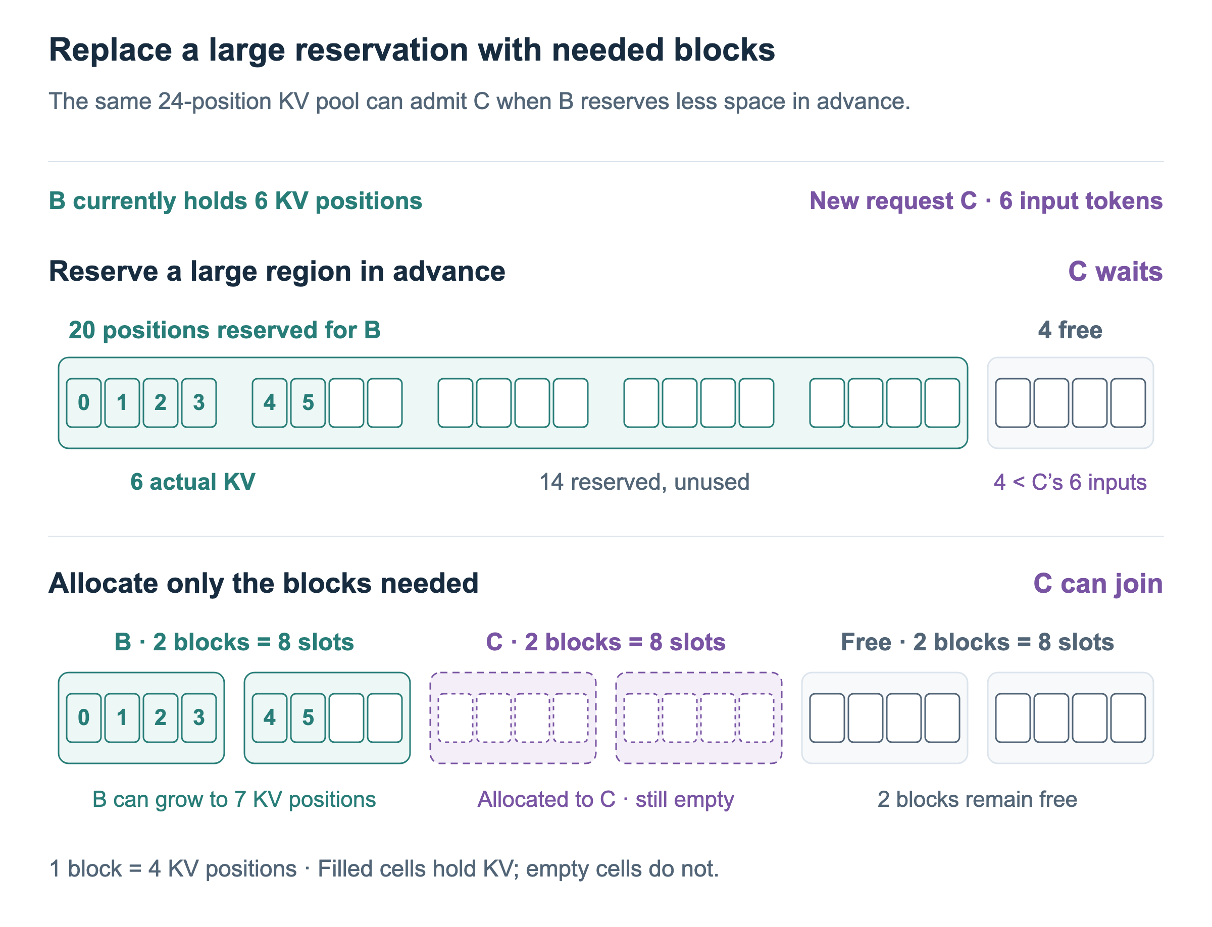
The lower half of Figure 1 allocates 8 slots each to B and C, or 16 in total, with 8 still free. By not tying up all the space B might need much later, the engine can make room for C. If B grows longer, it can receive additional blocks then.

Here, allocating space and computing KV are separate operations. C’s dashed blocks do not yet contain KV. Its input must pass through the model before KV is written into that space. After B and C finish the next execution, the actual KV will occupy 7 + 6 = 13 positions, leaving 3 of the 16 allocated slots empty.

Blocks can still leave empty slots in the last block. However, allocating only the blocks needed, as in this example, reduces the waste of reserving a large region for a request’s maximum length. The execution-token budget from the previous article is also satisfied, so C can run alongside B in this example.

Connect token order to storage locations

When blocks are allocated as needed, must each new block sit immediately next to the existing ones? That restriction would make expansion difficult again if another request occupied the neighboring space. Separating token order from physical memory locations allows the engine to use free blocks even when they are scattered.

First, let us move to the point after B and C have completed one execution. B has KV for 7 positions and C for 6. Dividing B’s KV into groups of four in token order puts positions 0 through 3 in the first block and positions 4 through 6 in the second. We will call these blocks, defined by order within a request, logical blocks. The first is L0 and the second is L1.

A physical block, by contrast, is actual storage in GPU memory. We will call the collection of physical blocks managed by the engine the block pool. The figure labels its six blocks P0 through P5.

B’s first logical block, L0, can be stored in P3, and its second, L1, in P0. The table recording which physical block holds each logical block is the block table.

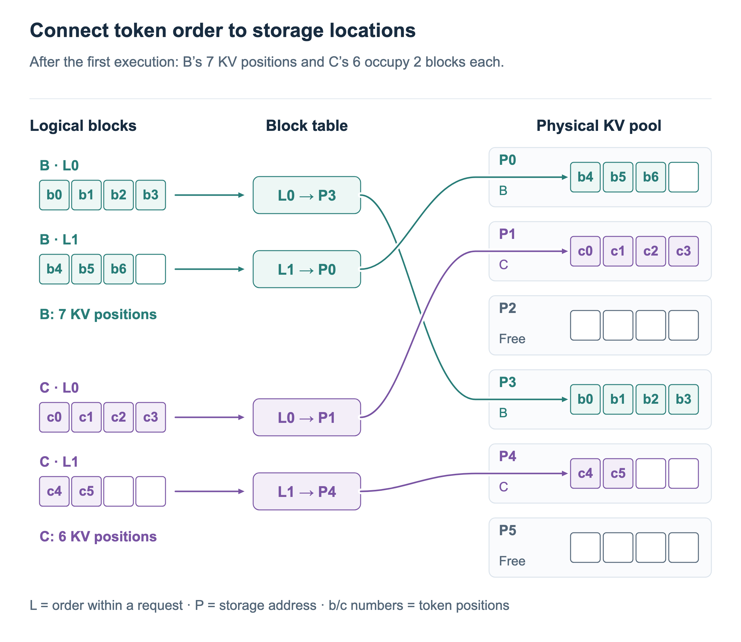
In Figure 2, B’s logical order is L0 followed by L1, while its storage locations are P3 followed by P0. C uses its own table to find P1 and P4. The logical blocks on the left and physical blocks on the right show the same data from different perspectives; they do not represent two stored copies of the KV.

For example, let us locate B’s KV for position 6. With a block size of 4, 6 ÷ 4 gives a quotient of 1 and a remainder of 2. This means the third slot in logical block L1. The table maps L1 to P0, so the computation can read the corresponding slot in P0. Both block indices and positions within blocks start at 0.

B's token position 6
→ logical block L1, position 2 within the block
→ look up L1 → P0 in the block table
→ KV at position 2 of physical block P0

Because the block table maintains this mapping, a request’s entire KV does not need to occupy one large contiguous region. The figure omits detailed storage layouts for individual layers and attention heads to focus on this correspondence.

Grow the allocation as generation proceeds

Now let us see how storage grows as B continues generating. B stores KV for 4 positions in P3 and 3 in P0. Its last block, P0, has one empty slot. This figure focuses on B’s changes while holding C’s KV at 6 positions.

When B processes its next input, the token at position 7, it can write KV into that empty slot. Its stored KV grows from 7 to 8 positions without needing another block. The logical-to-physical block mapping also stays the same.

When it processes the following input at position 8, both existing blocks are full. The engine then allocates a free block, P5, and adds L2 → P5 to the table. The new input’s KV is written into the first slot of P5.

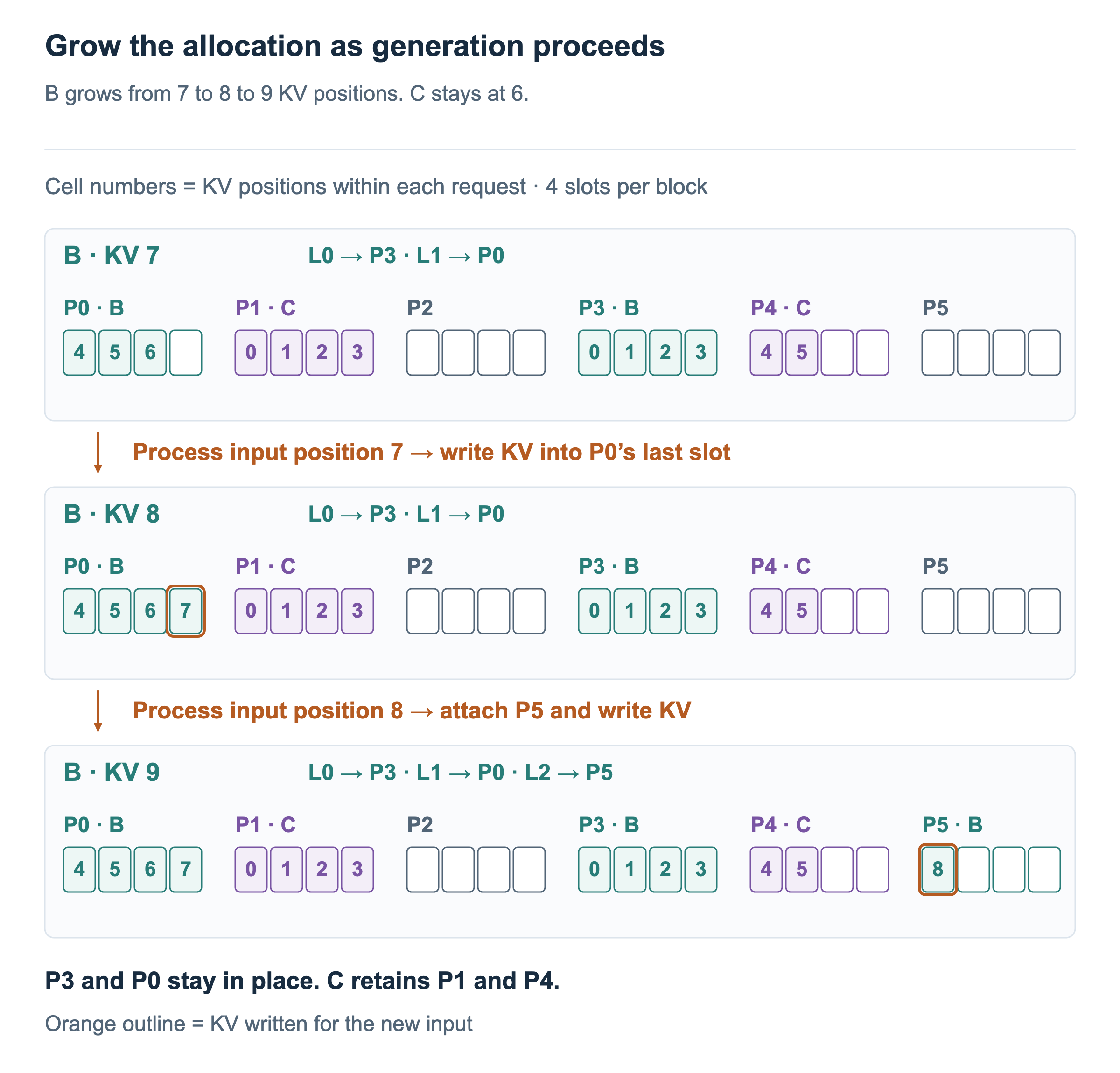
In Figure 3, only the last empty slot and one new block change. B’s past KV does not need to be copied into a larger contiguous region, and C retains P1 and P4. Storage grows in units of blocks, rather than by expanding the entire request’s allocation as one region.

The boundary for KV computation remains the same as before. When an execution ends and the next output token is selected, that output does not yet have KV. Its KV is created when the token is processed as the next execution’s input. The counts of 7, 8, and 9 in the figure therefore refer to KV positions stored after input processing.

The scheduler’s memory check can now be described more concretely. If the last block has an empty slot, the new input’s KV can be written there. Otherwise, the engine must check whether another block can be allocated. For a new request, it checks how many blocks are needed for the input context. Allocation can begin without knowing the output’s eventual full length.

Compute attention over scattered KV

Once storage is allocated in separate blocks, attention execution must understand that layout too. A computation that assumes one contiguous KV array cannot locate the data the request needs.

PagedAttention computes attention by using the block table to access KV blocks stored in separate locations. The block table identifies where data is stored, and the request’s valid context length determines which slots to use. The engine’s block management and this computation must work together. The PagedAttention paper describes both KV management and attention execution.

Let us continue with B processing input position 8. The Q computed from the current input uses KV for B’s positions 0 through 8, or 9 positions in total. This includes the current input’s own KV. In logical order, P3 holds 4 of these positions, P0 holds 4, and P5 holds 1.

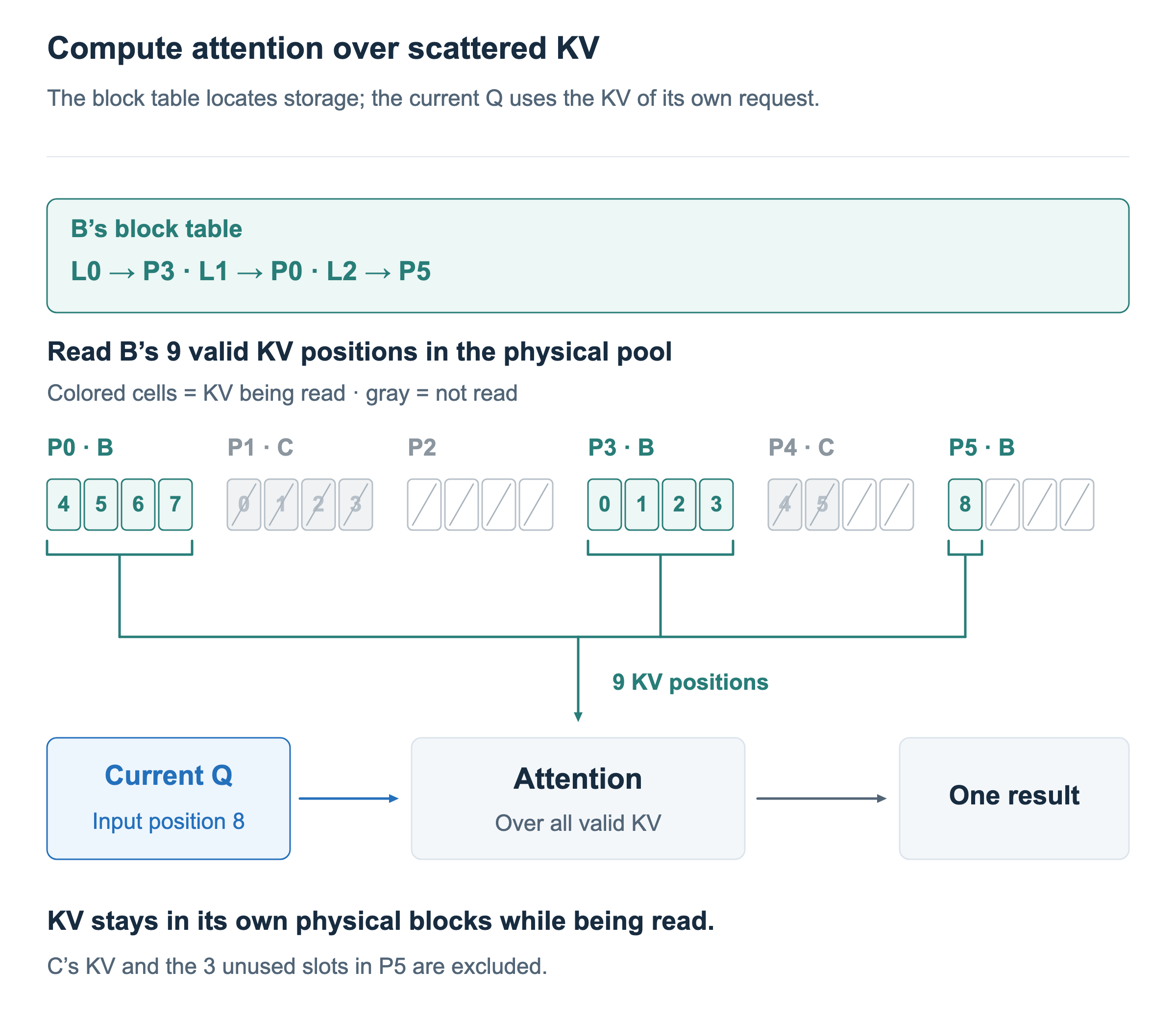
The connections in Figure 4 show which KV participates in attention. They do not represent a step that first gathers scattered KV into a separate contiguous buffer. KV is read while remaining in its own physical blocks. P1 and P4, which hold C’s KV, do not participate in B’s computation, and the three unused slots in P5 are also excluded.

Changing storage locations preserves the meaning of the attention computation. The weights determined from the relationship between the current Q and the keys must account for all valid keys across the three blocks. Combining V with those weights therefore produces attention over the request’s full valid context.

This allows KV storage to be allocated in separate blocks while preserving token order. It is the point where managing memory in blocks connects to actual model execution. We will leave the details of partitioning and combining computation inside the kernel outside this article’s scope.

Share common KV across responses

So far, separate requests B and C have held their own KV. Now consider generating multiple responses from the same input: two candidate answers to one prompt.

The input in this new example consists of 6 tokens, p0 through p5, and the block size remains 4. Because the same model processed the same input context, both responses start from the same input KV. This common initial part is called a shared prefix.

The simplest approach is to copy the input KV for each response. Each response needs 2 blocks, so two responses use 4 in total. But while both responses only read the same KV, the actual data need not exist in two copies. Pointing each response’s block table to the same physical blocks lets them share one copy of the KV.

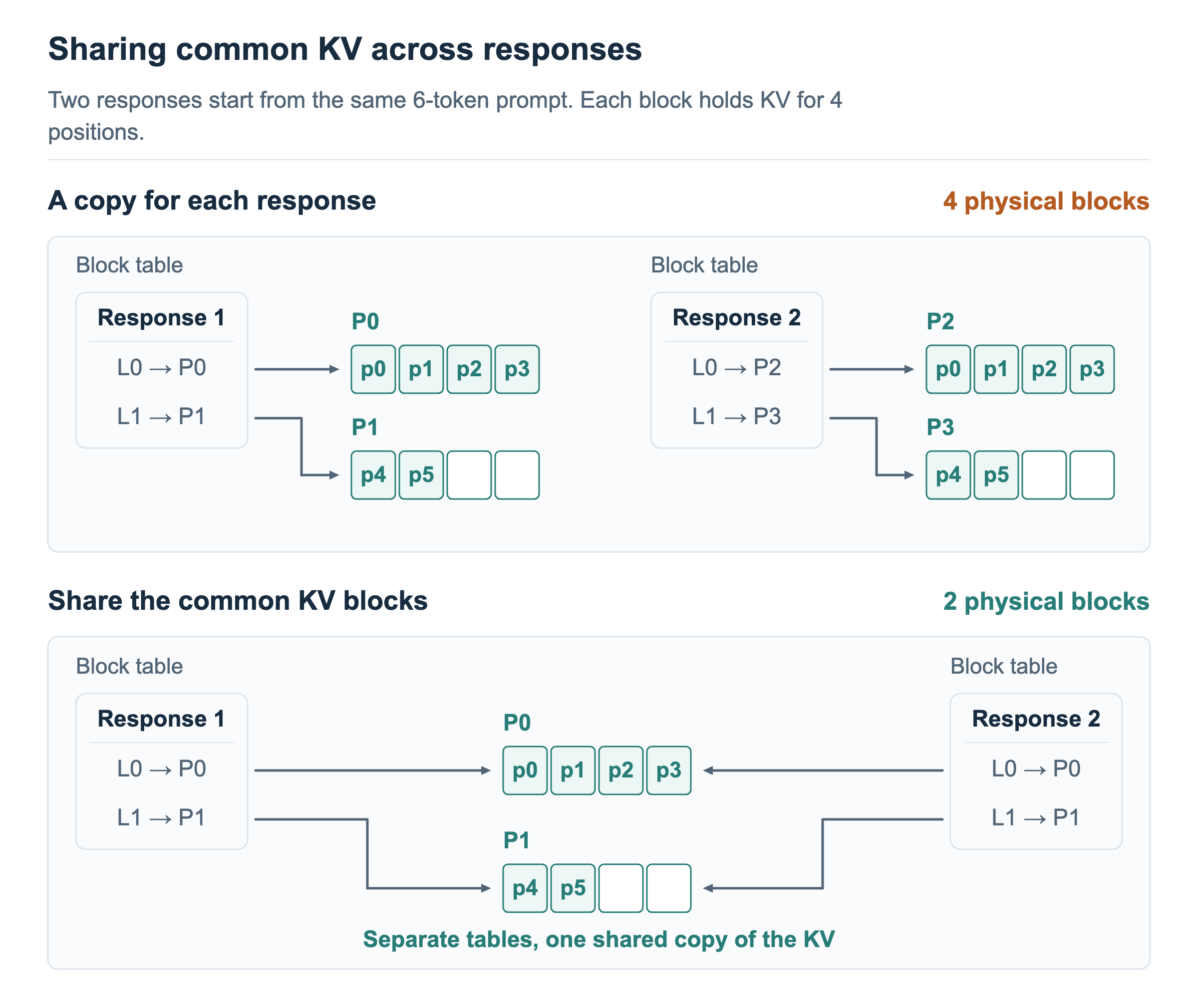
In the lower half of Figure 5, P0 holds KV for p0 through p3, and P1 holds KV for p4 and p5. Both responses map L0 to P0 and L1 to P1 in their own tables. The physical blocks holding the input KV decrease from 4 to 2.

Sharing is possible because the inputs match from the beginning of the context. The same word appearing by chance in two different contexts does not make its KV identical. What is shared is the storage for common KV. If subsequent inputs and Q differ between responses, each response still computes attention using its own Q and context.

Here we consider multiple responses that start together from the same input. A later article on prefix caching will examine how to find a shared prefix in a separately arriving request and reuse existing KV.

Split shared blocks when a write is needed

Both responses can point to the same blocks while only reading common KV. The situation changes when generation proceeds and new KV must be written.

In Figure 5, the last block, P1, holds KV for p4 and p5 and has two empty slots. Suppose response 1 processes a new input a0 and response 2 processes b0. If both keep sharing P1 and write into its next empty slot, they will write different KV into the same memory location. Even an empty slot is one physical space referenced by both responses, so it cannot hold their KV separately.

The engine must then copy the shared block that needs a write and point the writing response’s table to the new block. This approach, copying shared data when it actually needs to be modified, is called copy-on-write.

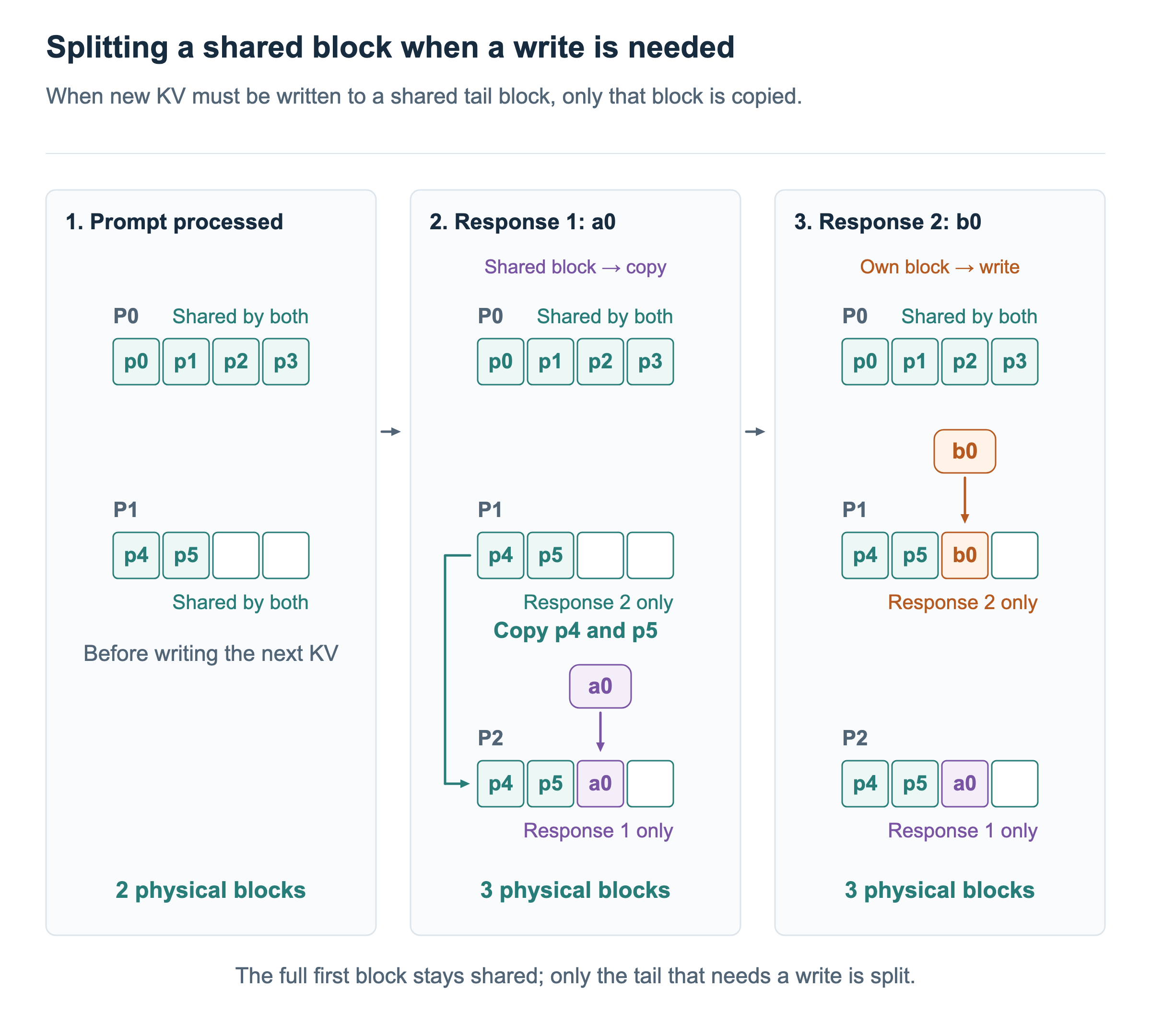
Let us follow the changes in Figure 6.

1. The common input has been processed. Both responses point to P0 and P1. There are 2 physical blocks in total.
2. Response 1 processes a0. The engine copies P1 to a new block P2, preserving the existing KV for p4 and p5, and changes response 1’s table to L1 → P2. The new KV computed from a0 is written into the next slot of P2. Response 2 still points to P1.
3. Response 2 processes b0. Only response 2 now uses P1, so another copy is unnecessary. It writes b0’s KV into the next slot of P1.

After the split, both responses still share P0 because its common input KV does not need to change. Each response holds its own last block for the differing part, bringing the total to 3 physical blocks. This is fewer than the 4 needed if each response had its own complete copy from the start.

The copy is not triggered by the mere selection of different output tokens. It is needed when those tokens are processed as subsequent inputs and new KV must be written into a block still referenced by multiple responses. If a shared block is already full, it can remain shared while each response receives a new block for its next positions.

Return blocks after a request ends

To manage sharing, the engine must also know how many responses reference each physical block. This is its reference count. In the example above, P1’s reference count decreased from two to one, allowing response 2 to write its KV without another copy.

When a response ends, its block references are released. Shared blocks still used by other responses remain in place, while blocks with no remaining references can return to the free block pool. Other requests can later write their KV into that space. This example does not assume a cache policy that retains KV after completion.

Block allocation reduces large reservations for space that is not yet needed, while block sharing reduces the waste of storing multiple copies of the same KV. The space saved allows continuous batching to consider admitting more requests. However, as actual KV requirements keep growing, free blocks can eventually run out. The next article, When KV Capacity Runs Out: Pausing and Resuming Requests, examines which requests to pause and which state to preserve when that happens.