Batching and Scheduling

Prefill and Decode showed that computing new inputs from several requests together lets us reuse the same weights more extensively. Grouping the computation for several requests this way is called batching, and the group executed together is a batch. Even when requests share an execution, each keeps its own context and KV cache.

In a real service, requests arrive at different times and finish generating at different times. If we must wait until every request in the original group finishes, it is difficult to use the room left by requests that finish earlier. If we can change the group as execution repeats, new requests can take their place.

This article starts with the limitations of a fixed batch and examines how to choose requests for the next execution. It then explains which resources to check before adding a new request, and why reserving KV space that is not yet in use can make new requests wait.

Static batching and continuous batching

Suppose requests A and B start generating together in one batch. A finishes with a short answer, while B continues generating a long answer. Meanwhile, a new request C arrives.

The simplest approach starts the next group of requests after both A and B finish. We will call this approach, which adds no new requests to a group once it has started, static batching. Even after A finishes its computation, C must wait until B finishes. We can skip the computation for the completed A, but cannot put C’s computation in its place.

Generation does not end after a single model execution. It repeatedly selects the next token and runs the model again with that token as input. After one execution finishes, we can therefore remove the completed A and add C to form the next batch. This approach, which updates the set of requests between model executions, is continuous batching.

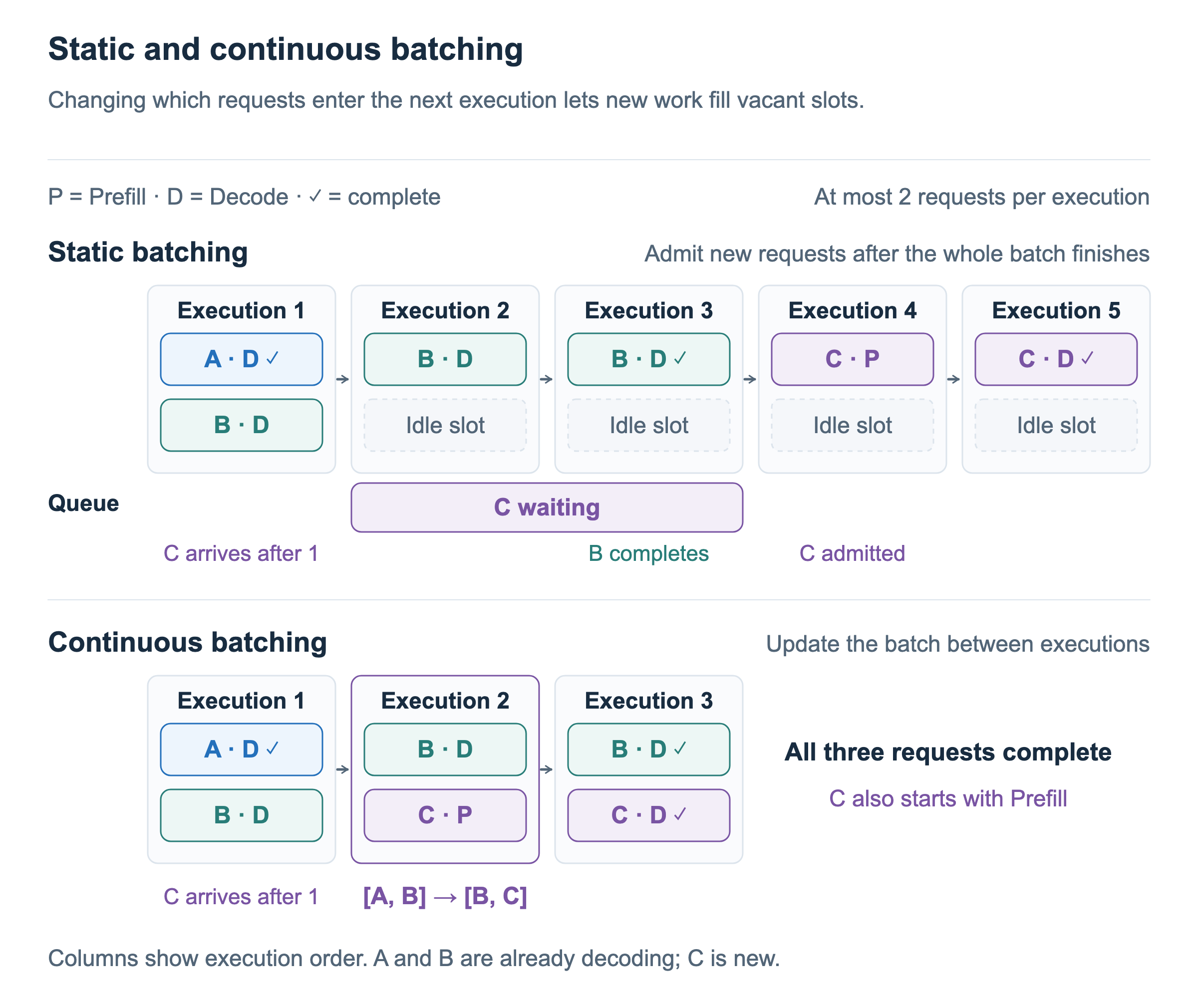
Figure 1 shows an example that executes at most two requests together. A and B are already in Decode, and C arrives just after A finishes in execution 1. With static batching, only B remains in executions 2 and 3. C starts in execution 4, after B also finishes.

With continuous batching, if resources are sufficient, the batch for execution 2 changes to B and C. B performs Decode because it is continuing generation, while C performs Prefill because its input context must be processed for the first time. In execution 3, both B and C perform Decode. Admitting a new request means starting with the first computation that request needs.

The cards here represent execution order. This article focuses on which requests to include in each execution. The key point is that updating the batch as shown lets C begin processing before B finishes. The ORCA paper also describes forming a batch at each repeated model execution, rather than waiting for entire requests to finish.

How the scheduler forms a batch

Continuous batching requires answering the same questions each time. Which requests have finished, which must continue generating, and which newly waiting requests can run alongside them?

Choosing the work to include in the next execution is called scheduling. The part of an inference engine responsible for this decision is the scheduler. Here, we are discussing how the engine selects requests and inputs to send to the model, rather than how instructions are assigned inside the GPU.

A newly arrived request first enters the waiting queue, a list of requests whose processing has not yet started. For requests that have already started, the engine keeps their generated tokens, completion status, KV stored on the GPU, and other state. The scheduler uses this information to form the next batch.

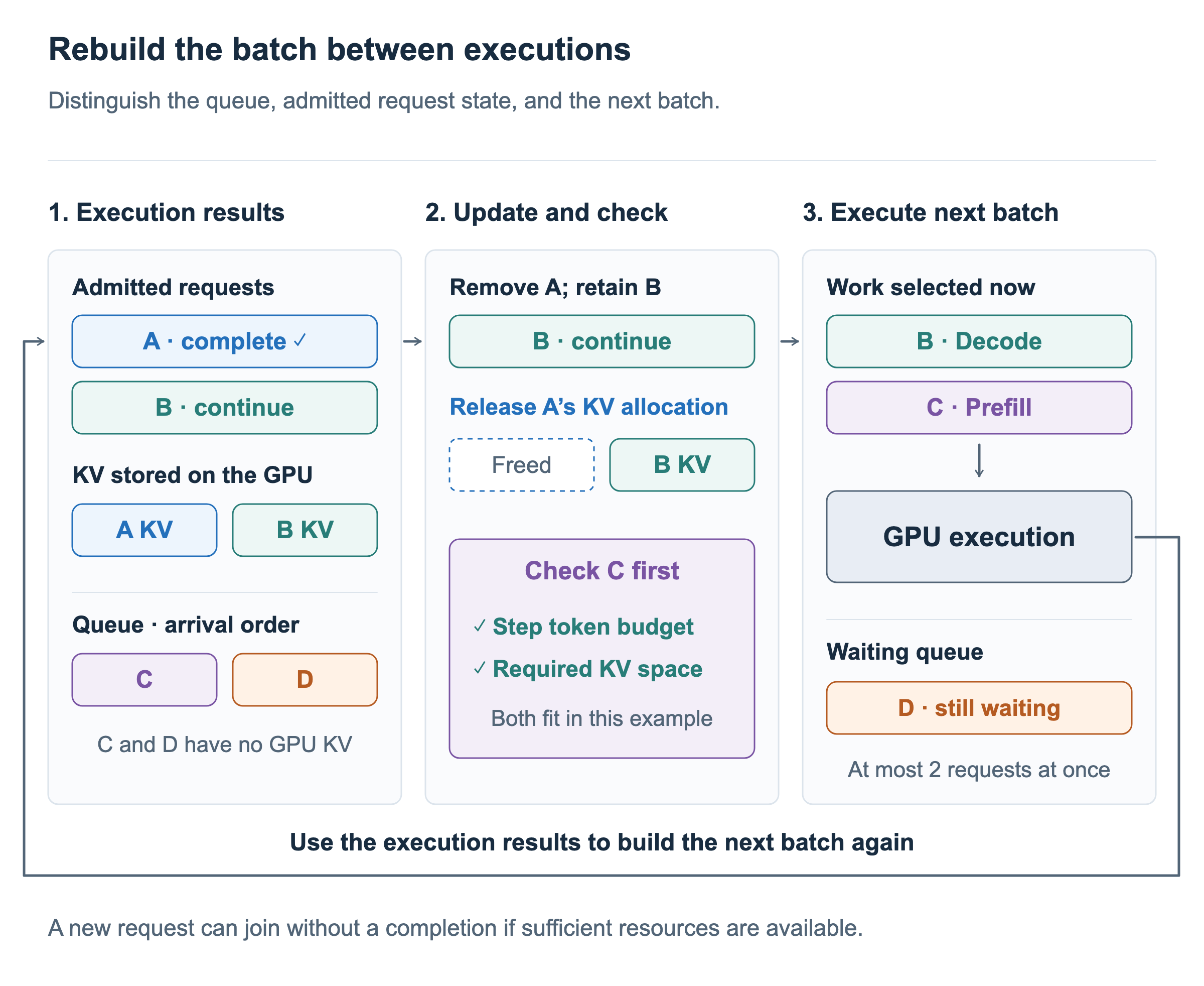
Let us walk through Figure 2 in order.

1. Check the execution results. A has reached its stopping condition, while B must continue generating the next token. C and D are in the waiting queue.
2. Clean up completed requests. Remove A from the next execution. The KV retained for A’s generation is no longer needed, so the space used exclusively by A is reclaimed. B must continue generating, so its KV is retained.
3. Consider admitting a new request. First prepare B’s next computation, then check whether resources are sufficient to include C as well. This example considers waiting requests in arrival order, an ordering called FCFS, or first come, first served.
4. Execute the selected batch. If resources are sufficient, execute B’s Decode and C’s Prefill together. The figure allows at most two requests, so D remains in the waiting queue. Once execution finishes, check the results again and repeat the same process.

A request does not have to finish before a new one can be admitted. Even if all ongoing requests continue generating, a new request can be added when resources are available. Conversely, even if A has finished, C may need too many resources to join immediately. A rule that simply adds one new request for each completed request is therefore insufficient.

What, then, should the scheduler check to decide whether resources are sufficient?

Resources needed for the next execution

The same number of requests can require different amounts of resources. B, which is in Decode, processes one new input in this execution, while the newly admitted C must process its entire input context. B’s existing KV must also remain in GPU memory.

We will therefore check the number of tokens processed now separately from the amount of KV retained after execution. The first determines how much new computation to include in this execution; the second describes the storage needed to maintain generation state.

Tokens processed in this execution

An engine can set an upper limit on the number of tokens included in one model execution. We will call this the execution-token budget. With a budget of 8, the total number of input tokens processed by the selected requests must be at most 8. This does not mean the GPU is physically limited to 8 tokens; it is a setting that limits the amount of work the engine executes.

The scheduler can count these tokens because it knows each request’s current state. One Decode execution for B has 1 new input. If C’s input length is 6, its Prefill processes 6 tokens. Selecting B and C therefore gives 1 + 6 = 7 tokens to process, within the budget of 8.

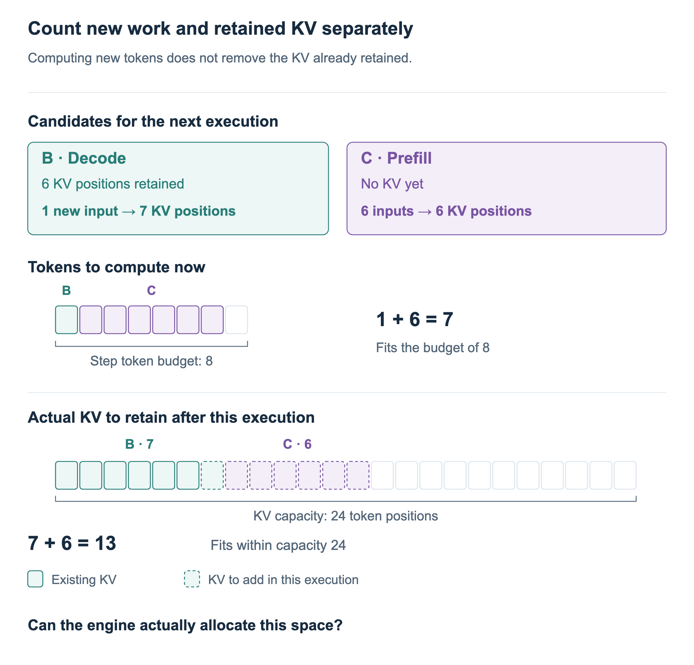
The upper bar in Figure 3 shows the 7 tokens processed now. We do not count B’s 6 previously processed positions again because their K/V is already cached. B’s Attention does, however, read the earlier KV. The token budget counts newly processed positions; it does not fully represent KV reads and Attention computation, which vary with context length. This is why equal token counts do not always mean equal execution times.

KV retained after execution

Now consider the lower bar in Figure 3. B already has KV for 6 positions. Processing one new input adds that input’s KV, bringing the total to 7. C processes its 6 inputs for the first time, creating KV for 6 new positions. The KV retained after execution therefore occupies 7 + 6 = 13 token positions.

The boundary of KV computation remains the same as in the earlier article. KV has not yet been created for the next output token that B will select from this execution’s result. Only the KV for the one position supplied as input is added, so B’s KV grows from 6 to 7 positions.

Actual memory is managed in bytes. Once the model, KV storage data type, and related details are fixed, we can calculate the memory needed to store one token position’s K/V across the layers. The engine determines how much memory it can use for KV after accounting for weights, computation workspace, and other needs, then checks the KV space required by each request.

Here, we assume the same model and KV storage format, and express space as the number of token positions whose KV it can store. The KV capacity of 24 in the figure is the space available for KV, not the GPU’s entire memory. These numbers illustrate the decision process rather than reproduce the settings of a particular engine.

The actual KV requirement is 13 positions, which fits within the total capacity of 24. But one more check remains: that much space must actually be allocatable to the requests. If some memory is already set aside for another request’s future generation, it may be unavailable to C even though no data has been written there yet.

Why reserve KV space in advance?

Before examining the space available to C, let us consider why space that is not yet in use might be set aside in advance.

The KV cache keeps growing as a request progresses. Even if B currently has KV for 6 positions, processing the next input increases it to 7, and continued generation requires more space. The input length is known from the start, but it is difficult to know exactly when the output will end before generation begins.

One approach is to allocate KV space in advance for the maximum length the request is allowed to use. For example, if the KV stored for the input and during generation is allowed to occupy at most 20 positions in total, we can allocate space for all 20 positions to B from the outset. Reserving space does not mean computing data in advance; it means setting aside memory for B’s future KV.

Within the chosen length limit, B then needs no additional allocation each time its KV grows. This is particularly easy to manage when a request’s KV is stored in one contiguous memory region: a sufficiently large region is allocated from the start. If only the currently needed size were allocated and another request occupied the adjacent space, expanding the same region could be difficult.

The maximum length, however, differs from the length at which a request actually finishes. If B finishes before using all 20 positions, the remaining space will have gone unused. While generation is still in progress, there is also space that has not yet been filled. This reserved space is one of the problems with earlier KV management approaches described in the PagedAttention paper.

Reserving a large region in advance is one way to manage KV. Not every inference engine must reserve space for the maximum length. Let us examine how this approach affects the processing of the next request.

Unused reservations make new requests wait

Figure 4 uses the same B and C whose KV requirements we calculated earlier. The KV capacity is still 24 positions. We now add the condition that B has already reserved space for 20 positions.

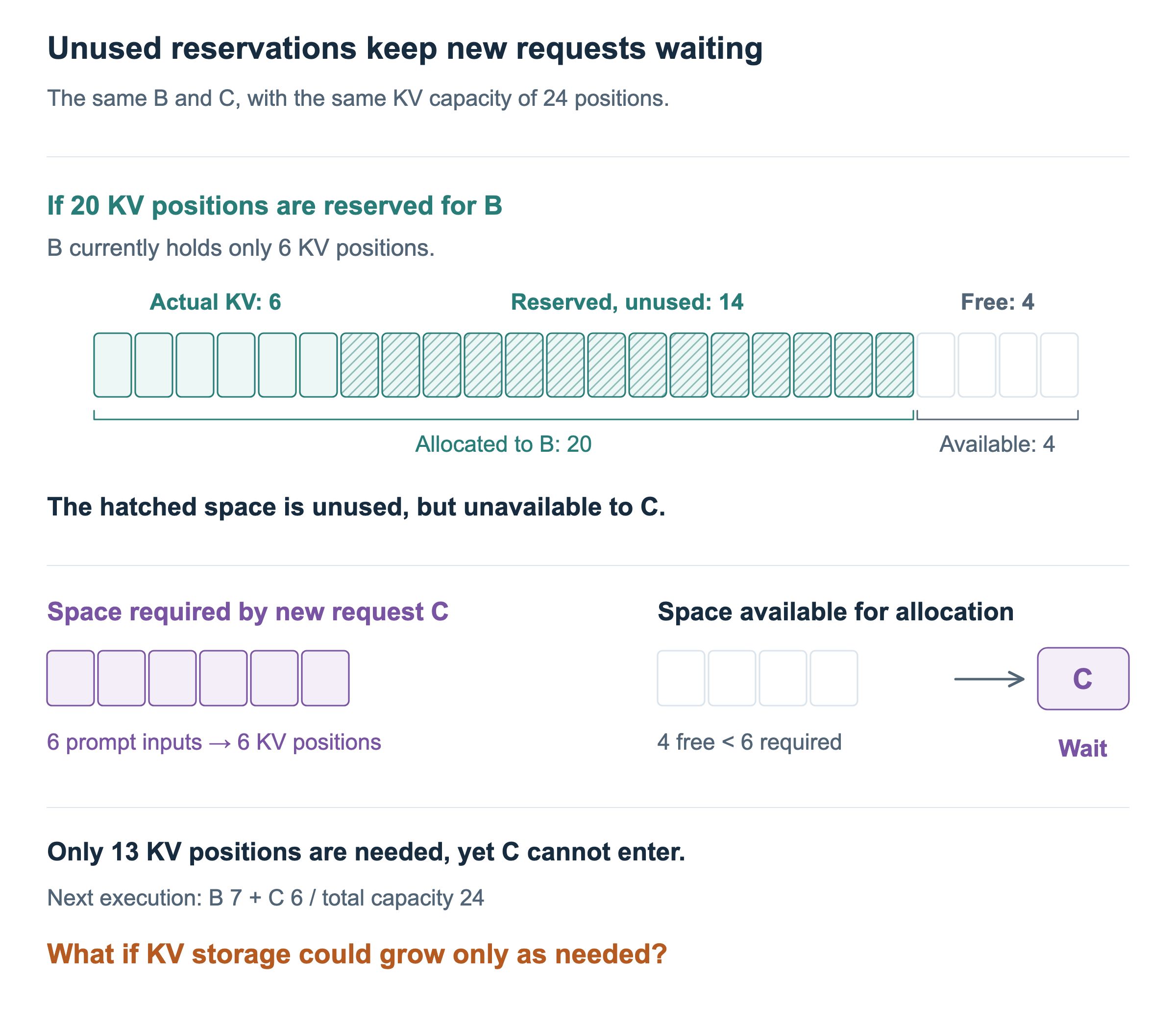
At the top of the figure, B stores actual KV in 6 positions. The 14 hatched positions are reserved for B but not yet used. Together, these 20 positions belong to B, leaving only 24 − 20 = 4 free positions that can be allocated to another request.

B can use its own reservation for the one additional position needed by its next Decode execution. C’s Prefill, however, needs 6 newly allocated positions. Only 4 are available to C, so C cannot be included. There is insufficient space to hold the KV for its input context even before considering additional room for its later generation.

Looking only at the actual data gives a different picture. As calculated earlier, the KV stored after executing B and C would occupy 13 positions, less than the total capacity of 24. C is waiting because unused space is tied up in B’s reservation, not because the two requests’ actual KV exceeds total capacity.

The scheduler therefore cannot stop at calculating token counts and KV requirements. It must also check whether the current memory management approach can actually allocate that space. C joins in Figure 2 because the required space can be allocated; Figure 4 shows the same admission blocked by reserved space.

Even if continuous batching lets us change the set of requests at each execution, large unused reservations make it difficult to admit enough new requests. Updating batch membership frequently and using KV space efficiently are problems that must be addressed together.

Could we allocate space as KV grows instead of reserving a large region for the maximum length? The next article, KV Cache Management and PagedAttention, examines how to allocate KV in small units and read a request’s KV even when its storage locations are not contiguous.