Shared Concepts · Hardware · 2026-09-18
TP: Split One Operation Across GPUs
Partition weight matrices by columns and rows, then connect these partitions in FFN and attention to avoid intermediate communication.
In data parallelism (DP), we replicated the model and assigned different inputs to different GPUs. Tensor parallelism (TP) divides computation for the same input across multiple GPUs. Several GPUs can cooperate even while processing a single request, and they can partition a single weight matrix between them. Here, a tensor means an array of values, such as a vector or matrix.
Splitting an operation reduces each GPU’s computation, but connecting the distributed results becomes important. Gathering the full result after every operation can spend substantial time on communication. We will first examine how the results differ when we split weight columns or rows. We will then connect the two approaches in FFN and attention to skip intermediate communication, and locate the communication that remains across a transformer layer.
The figures show a forward pass in which two GPUs process the same input. Blue indicates GPU 0’s share; orange indicates GPU 1’s. Use Next to advance the computation. Matrix grids without numbers show shapes and partition boundaries rather than values. Click a figure to open the original at a larger size.
Splitting Columns to Complete Output Shards
Start by dividing one matrix multiplication, Y = XW, between two GPUs. X is the input, W the weights, and Y the output. In the figure, X is a 2×4 matrix containing two tokens, each with four feature values. Each row represents a token, and each column a feature. Remember that the GPUs share the computation for the same two tokens, rather than handling different tokens.
W is a 4×4 matrix. Each column of W uses all four input features to compute one output feature. Splitting W by columns therefore lets the GPUs handle different output features. GPU 0 stores the first two columns, and GPU 1 the last two. Both GPUs hold the full input X.
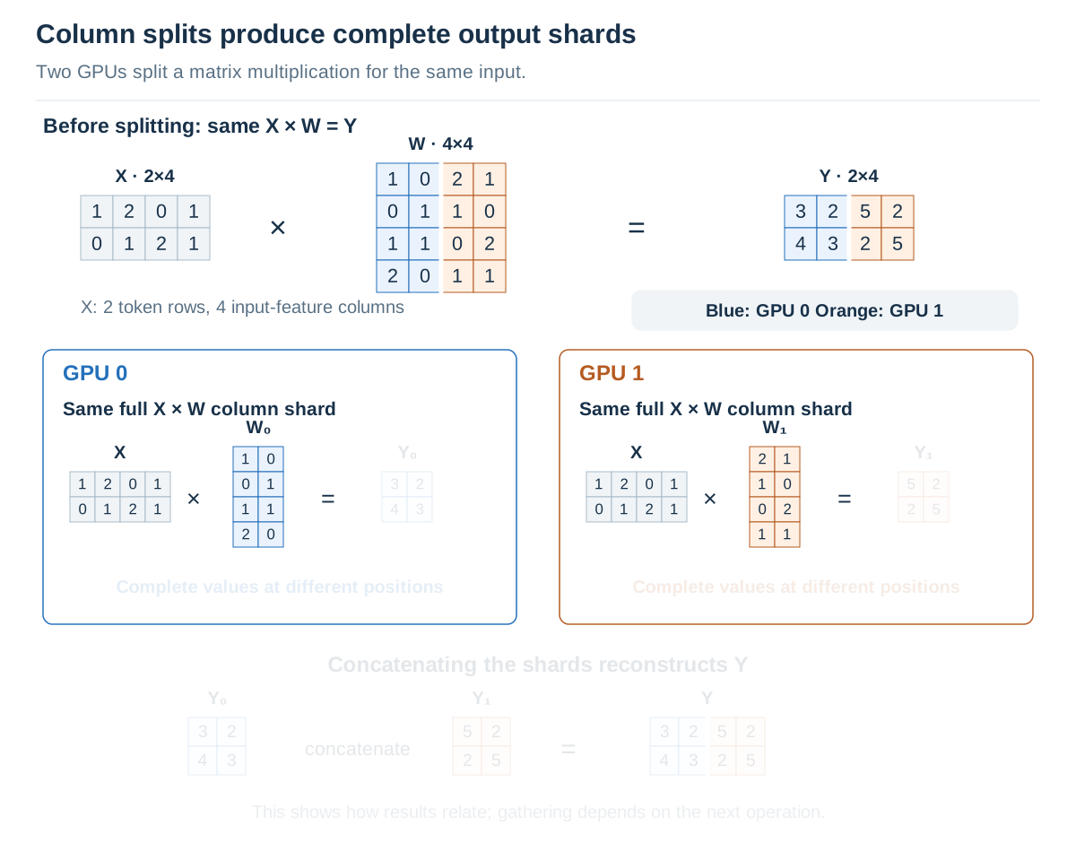
1. Partition the matricesView the completed figure
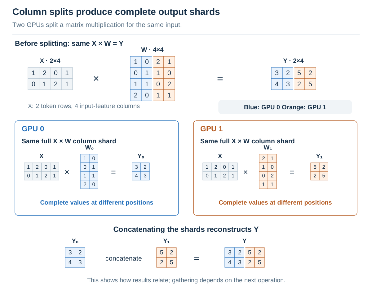
Use Next to follow the computation. Click the figure to enlarge it.
The first token’s input is [1, 2, 0, 1], and its complete output is [3, 2, 5, 2]. GPU 0 computes the first part, [3, 2], while GPU 1 computes the last part, [5, 2]. Each value already includes all the multiplications and additions needed for that output feature.
Column partitioning thus produces complete output shards at different positions. To reconstruct the full Y, place the shards side by side along the column dimension, rather than adding them. The second token is computed in the same way.
This does not mean the implementation must gather the shards immediately. If the next operation needs all of Y on every GPU, All-Gather can collect them. If it can start using only the local shard, the results can remain partitioned. The figure’s final step shows the relationship between the shards and the full output; it does not require communication at that point.
Splitting Rows to Compute Partial Output Sums
Now partition the same X and W in another direction. Place the first two rows of W on GPU 0 and the last two on GPU 1. Because W’s rows correspond to input features, split X’s feature columns accordingly. GPU 0 uses the first two features of each token, and GPU 1 the last two. “Row partitioning” here refers to the rows of the weight matrix W, not to splitting input tokens.
Computing one output value requires adding the products for all input features. Each GPU now handles only some of those features, so its result is not yet the complete sum. We will call this a partial sum.
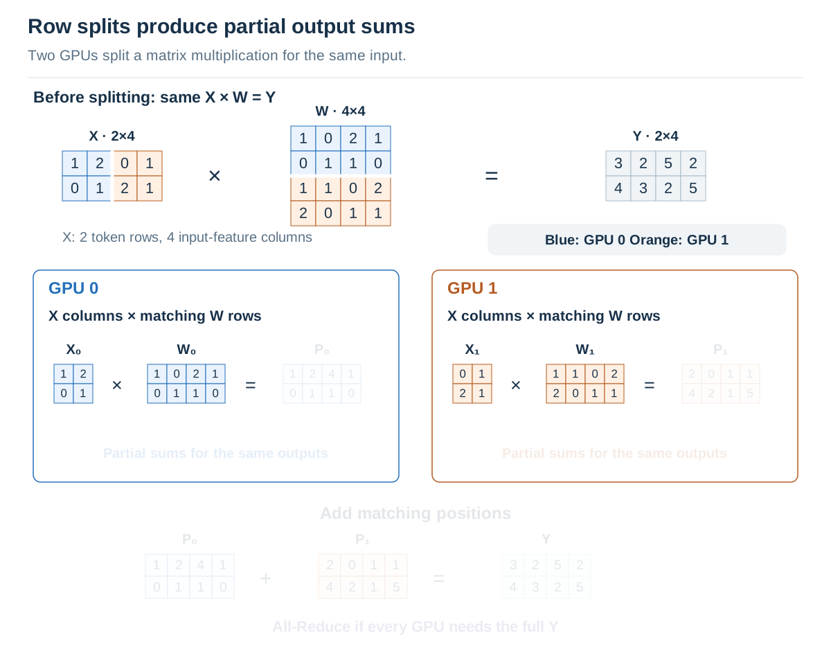
1. Partition the matricesView the completed figure
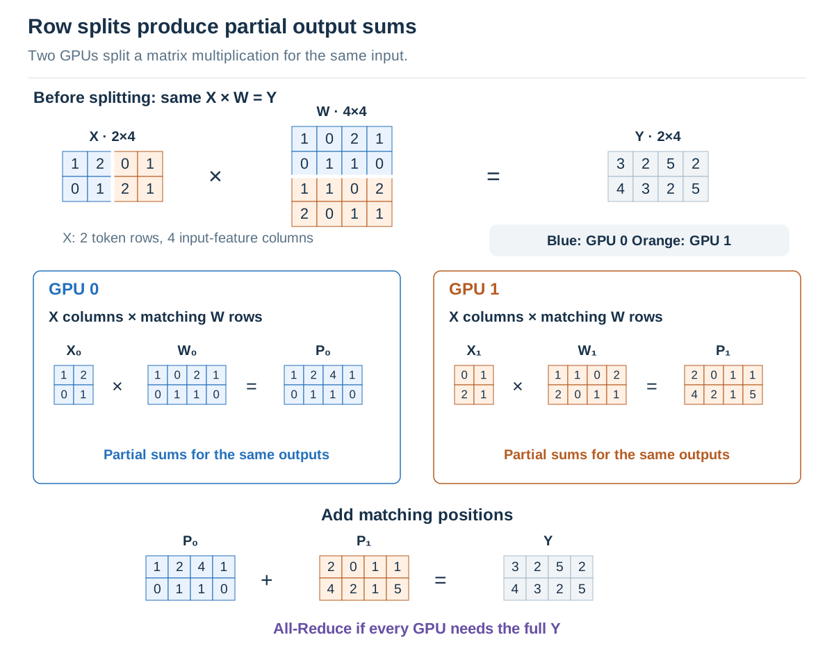
Use Next to follow the computation. Click the figure to enlarge it.
For the first token, GPU 0’s partial sum is [1, 2, 4, 1], and GPU 1’s is [2, 0, 1, 1]. Adding matching positions produces the original output, [3, 2, 5, 2]. For example, the first output value, 3, comes from adding GPU 0’s 1 to GPU 1’s 2.
Unlike column partitioning, each GPU’s result has the same shape as the full Y. But having the same shape does not make it a complete result. Each result includes only some input features, so concatenating the two results would not reconstruct the original matrix multiplication. Matching positions must be added.
If both GPUs need the summed result, we use All-Reduce. This collective adds values at matching positions across GPUs and returns the complete result to every participant. The examples below use it to prepare the full output on each GPU.
We can now distinguish the two partitions. A column split completes different pieces of the output; a row split produces partial sums contributing to the same output positions. Next, we will use this distinction to connect two operations.
Connecting Column and Row Partitions in an FFN
A transformer’s feed-forward network (FFN), also called an MLP, transforms each token’s features. We will use a basic form with an activation function between two linear transformations, or Linear layers. The first Linear expands the feature dimension, and the second reduces it again. The activation applies a nonlinear transformation to the values between them.
We can write this as Y = f(XU)V: multiply X by the first weight matrix U, apply activation f, then multiply by the second weight matrix V. The figure expands four input features to eight intermediate features, then reduces them to four again. Bias terms are omitted for simplicity.
Splitting the first weight matrix U by columns partitions the intermediate result along the feature dimension. GPU 0 computes the first four features, and GPU 1 the last four. Each feature value is already complete, without needing to add a result from the other GPU.
Before moving to the second Linear, we must apply the activation function to these intermediate values. Here, we use an elementwise activation that transforms each value independently, such as GeLU. Transforming one feature value does not require the other features, so GPU 0 can apply the activation to its first four features and GPU 1 to its last four. This produces the same result as gathering all eight features, applying the activation, and splitting them again. The intermediate values can therefore remain partitioned across GPUs as we move to the next Linear.
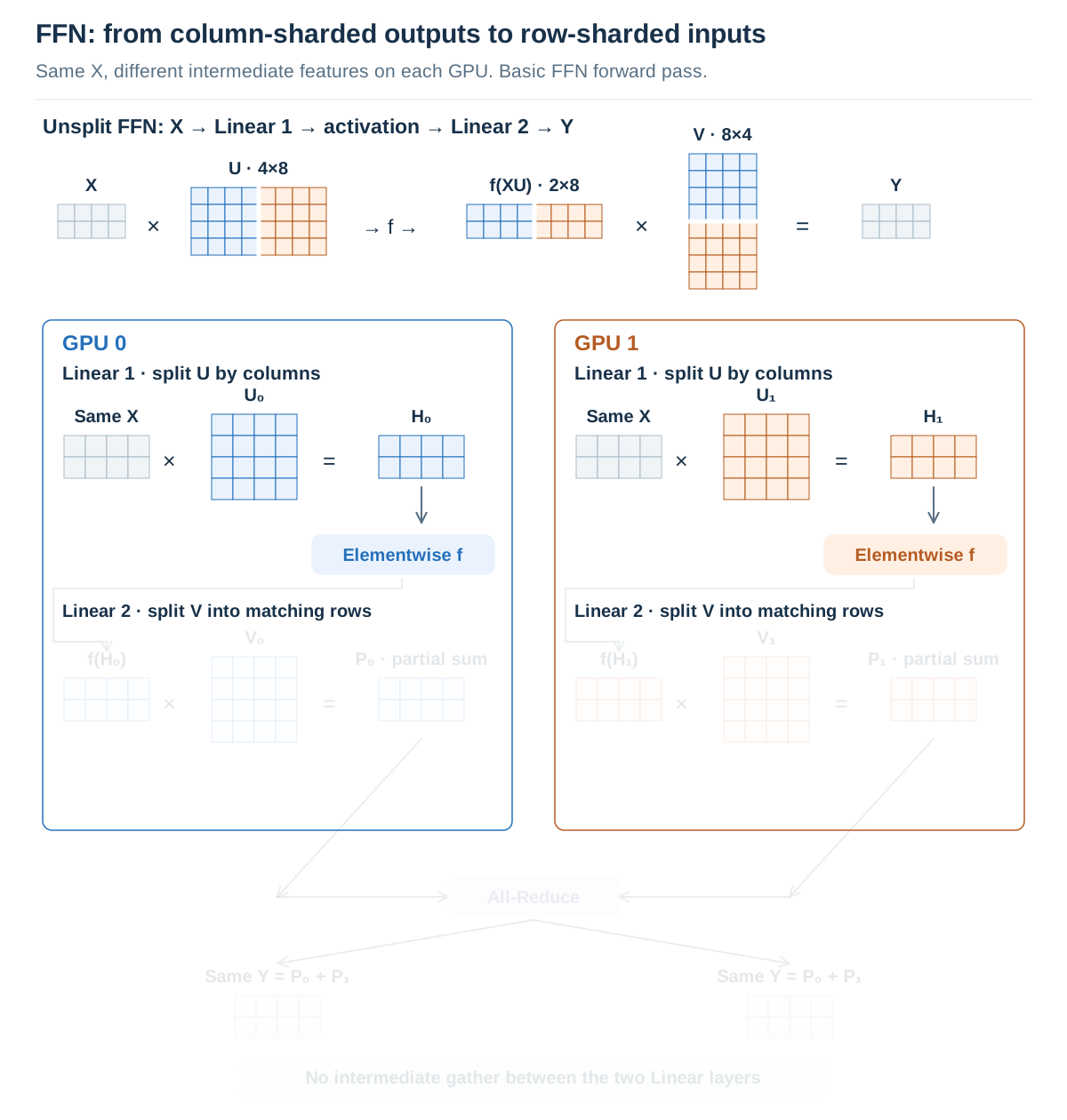
1. First Linear and activationView the completed figure
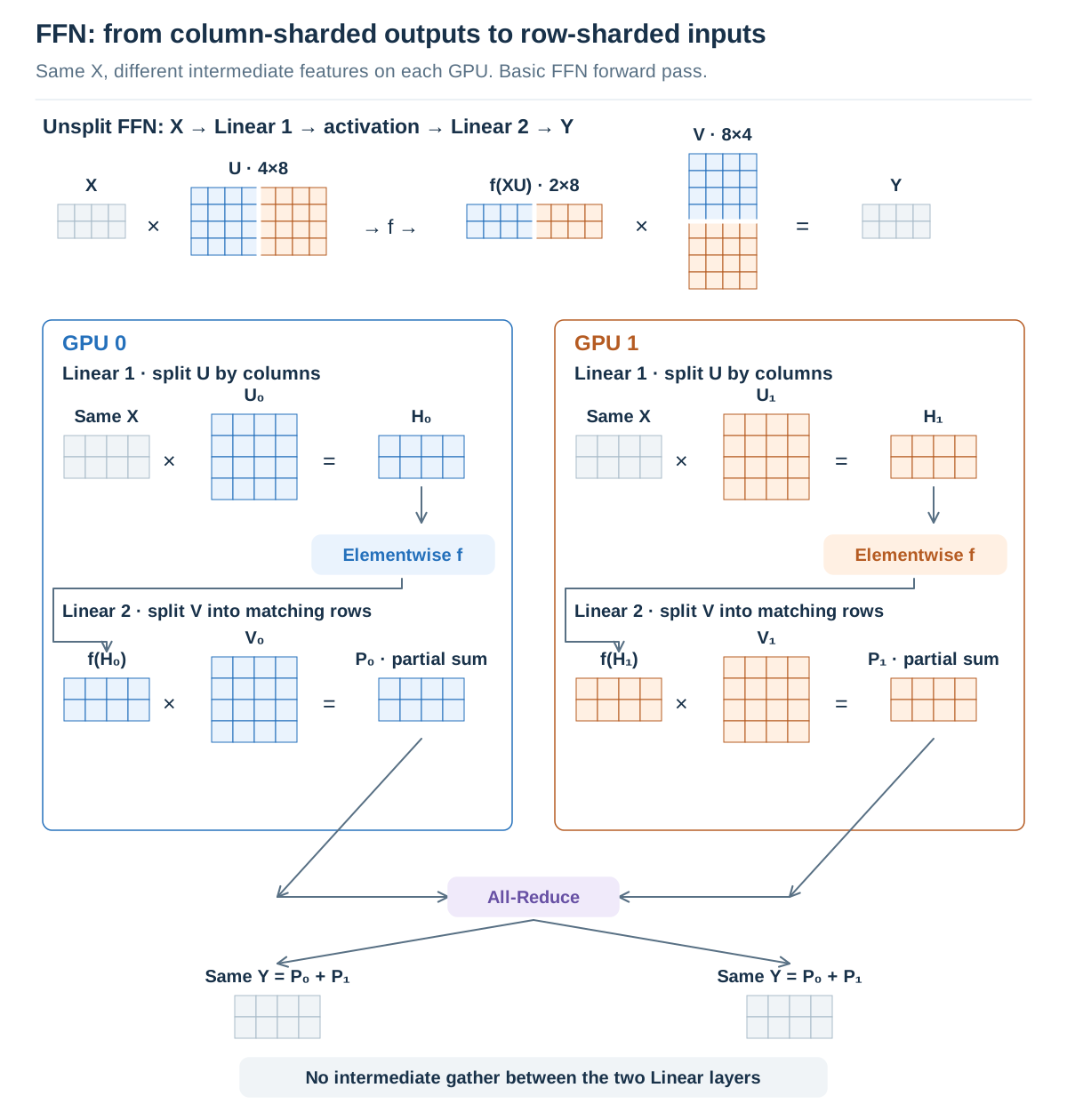
Use Next to follow the computation. Click the figure to enlarge it.
The key comes next. Split the rows of the second weight matrix V to match the intermediate features already held by each GPU. GPU 0 receives the rows corresponding to the first four features, and GPU 1 those for the last four. Each GPU can then compute the second matrix multiplication using only its local intermediate values and V shard.
Because this is a row-partitioned operation, the results are partial sums. A final All-Reduce adds them so both GPUs receive the complete Y.
Splitting the first Linear by columns and the second by rows lets us skip gathering the full intermediate values between them. We align the weight partitions so the next operation can directly use the shards produced by the first. There is no need to gather the intermediate result only to split it again.
Keeping Attention Computation Local to Each Head
Attention also contains linear transformations for its input and output. Creating Q, K, and V from input X is called the QKV Projection. Transforming the heads’ attention results into the final output features is called the Output Projection. Here, a projection means transforming features by multiplying them by a weight matrix.
In ordinary multi-head attention, each head computes attention using its own Q, K, and V. If we place all the values needed by one head on the same GPU, that head’s attention can be computed without the other GPU’s head result. Each GPU handles one of the two heads in the figure.
To achieve this, split the columns of WQ, WK, and WV along head boundaries. Both GPUs use the same X, but produce Q, K, and V for different heads. Each GPU’s Q, K, and V include both tokens needed by its head. This differs from splitting the tokens in half.
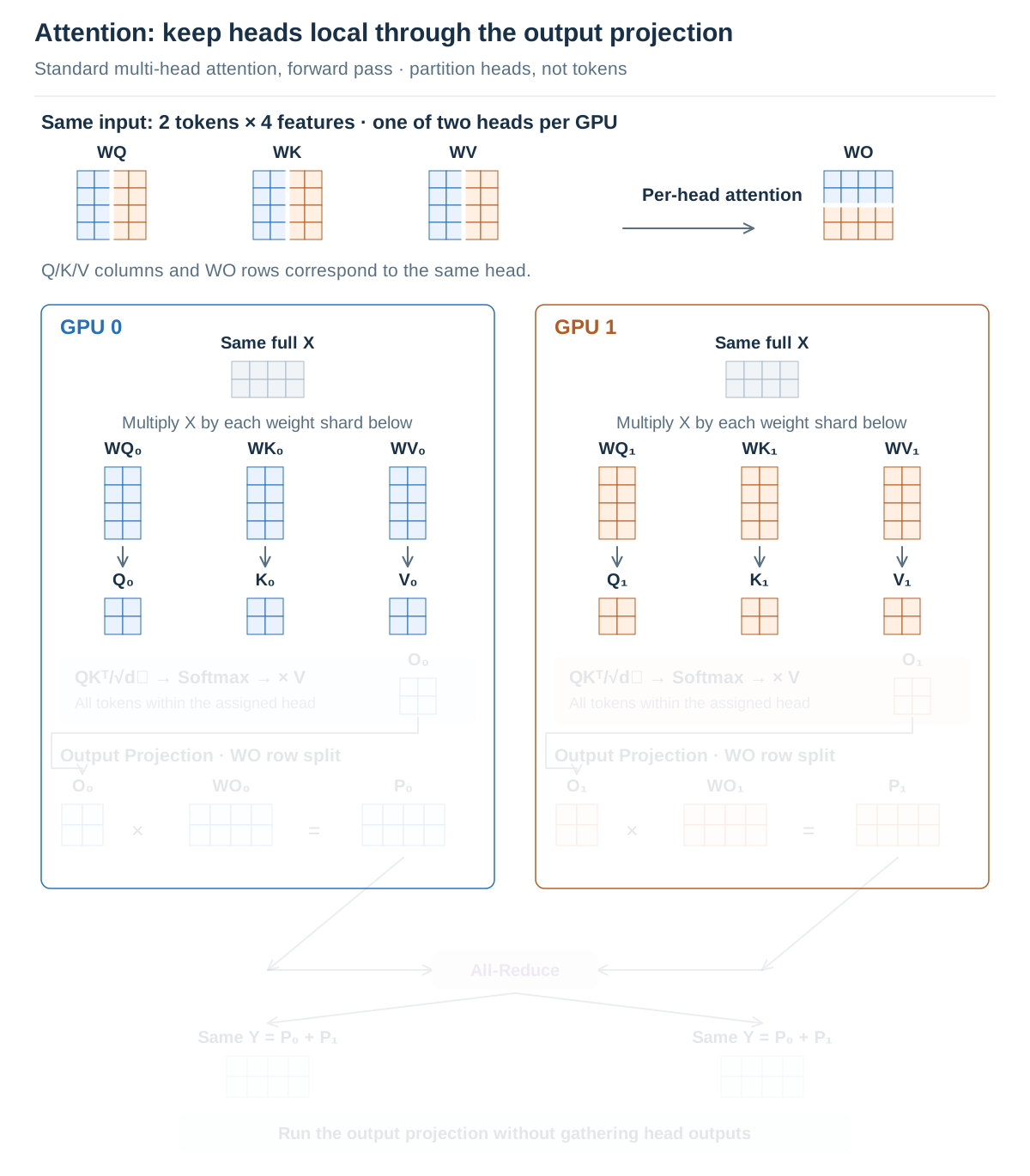
1. Q/K/V projections by headView the completed figure
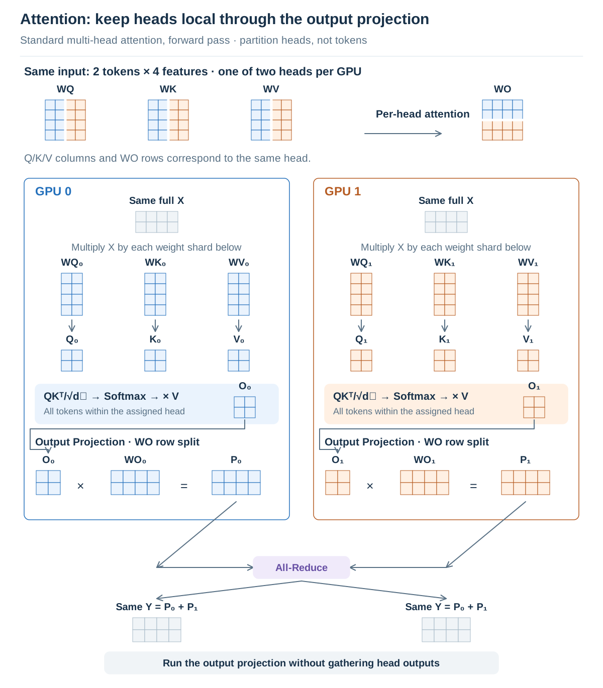
Use Next to follow the computation. Click the figure to enlarge it.
Each GPU computes scores with its Q and K, applies Softmax, and forms a weighted sum of V to produce its head output. Call GPU 0’s output O₀ and GPU 1’s output O₁. Up to this point, each head’s computation stays within its GPU.
We could now gather all head outputs and perform the Output Projection, but, as with the FFN, we can skip that gather. Partition the rows of the output weight matrix WO to match the head output on each GPU. GPU 0 multiplies O₀ by its corresponding WO rows, and GPU 1 multiplies O₁ by the remaining rows. These results are partial sums for the same final output, so we add them with a final All-Reduce.
Concatenating all head outputs and multiplying by WO gives the same result as multiplying each head output by its matching WO shard and adding the results. We can therefore continue through the Output Projection without gathering head outputs in between.
The computation in the middle differs between FFN and attention, but the connection pattern is similar. Split the first projection by columns, continue with independent computation on each GPU, then split the output projection by rows and sum the final partial outputs. This does not mean the entire attention block consists of only two matrix multiplications. Score computation and the weighted sum of V also occur between the Q/K/V projections and the output projection.
The figure assumes ordinary multi-head attention with Q, K, and V for each head. Architectures that share K and V across multiple heads require additional consideration of which heads and data to place together or replicate.
Locating Communication Across the Whole Layer
Now connect these pieces into two GPUs jointly processing one transformer layer. The figure uses a Pre-Norm structure, with normalization before attention and FFN. Normalization adjusts the scale of input features, while a residual connection adds a block’s input to its output.
Both GPUs hold the same full input X at the layer entrance. After normalization, they independently perform the QKV projections, per-head attention, and output projection. All-Reduce then adds their partial sums and prepares the same complete result on both GPUs. Each GPU adds the input it retained to compute the residual connection.
The FFN repeats this pattern. After normalization, each GPU computes the first Linear, activation, and second Linear locally, then uses All-Reduce to sum the results. After adding the residual, both GPUs hold the same layer output and proceed to the next layer.
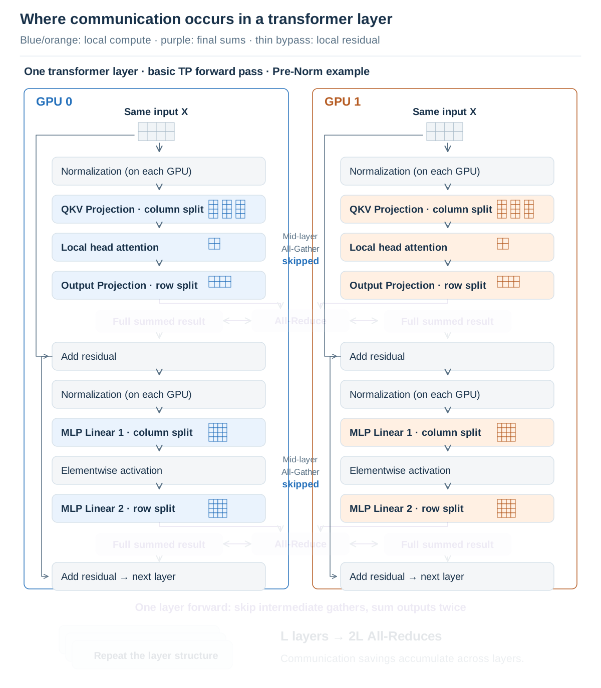
1. Each GPU's computation pathView the completed figure
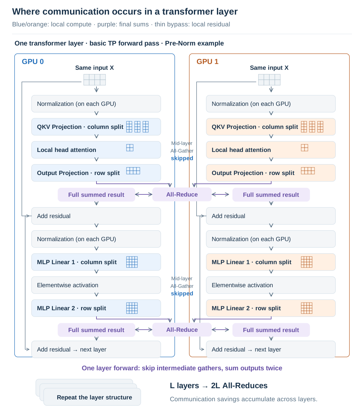
Use Next to follow the computation. Click the figure to enlarge it.
Thus, one layer in the depicted basic TP layout needs two All-Reduces in its forward pass: one after attention’s output projection, and one after the FFN’s second Linear. Connecting column and row partitions avoids gathering attention head outputs and FFN intermediate features. This is the basic TP arrangement described in the Megatron-LM paper.
A transformer stacks many such layers. With L layers of the same structure, these two sums alone repeat as 2L All-Reduces in the forward pass. The benefit of removing intermediate communication within one layer also accumulates across layers. This is why partitioning one matrix multiplication well is only part of the task: its shards should remain usable by the next operation. This count covers only the forward pass of the two blocks shown; it excludes communication for backpropagation, embeddings, and other parts of the model.
TP can reduce each GPU’s burden by partitioning the weights and computation for one input. However, execution time is not guaranteed to shrink in proportion to the partitioning. Communication and waiting take time, and splitting into very small matrices can reduce each GPU’s compute efficiency. Check whether the saved compute time is large enough to outweigh communication costs, and whether the overall completion time for the same input actually decreases.
The normalization and residual sections in the figure also show both GPUs storing the same full inputs and intermediate values and performing the same computation. Partitioning weights does not partition all data. We will examine how to split some of these remaining replicated intermediate values along the token dimension when we discuss SP.