DP: Replicate the Model, Partition the Inputs

A straightforward way to use more GPUs is to prepare more copies of the same model. It resembles several people using the same tools to handle different jobs. This is data parallelism, or DP.

We will first examine model and input placement, then compare inference with fixed weights against training that updates them. Finally, we will examine how dividing inputs increases request throughput in inference and data throughput in training. The examples use an ordinary dense model that applies the same set of weights to each input token.

Replicating the Model and Dividing Inputs

Assume four GPUs each hold the entire model W. Send request A to GPU 0, B to GPU 1, and so on. Each GPU runs its own request through the model from beginning to end.

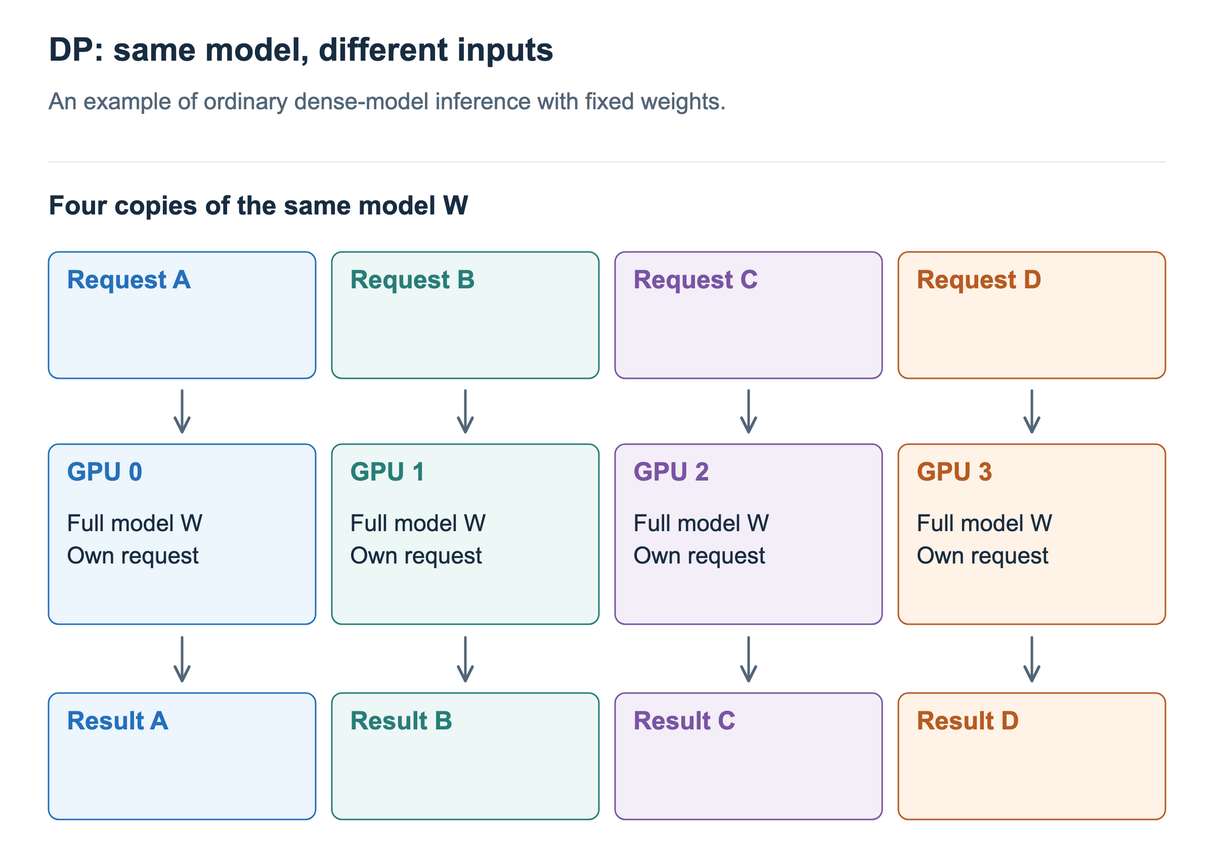
What is partitioned is the input assigned to each replica, rather than model layers or weight shards. Basic DP therefore does not reduce per-GPU weight memory. It cannot make a model that exceeds one GPU’s capacity fit in that placement.

If the model fits and there are enough requests, multiple GPUs can work at once. This does not restrict each GPU to one request: each replica may batch multiple inputs. Batch size and input distribution affect the resulting throughput.

Distributing Inference Requests

Inference computes results using prepared weights. With fixed weights and independent requests, replicas do not need to All-Reduce every computed result: request A does not depend on request B’s output.

A dispatcher must instead choose a replica for each request. Round-robin assignment is possible, but different input and output lengths mean equal request counts need not represent equal work. Sending more long requests to an already busy GPU can increase queueing.

If a request spans multiple computations, its state must also be managed. A request generating tokens one at a time can reuse previously computed information, so sending each next computation to an arbitrary replica is not sufficient. State must remain available or be transferred appropriately. vLLM’s data-parallel deployment documentation gives practical request-distribution examples. Unlike our independent dense replicas, configurations involving MoE may introduce additional communication relationships.

Combining Gradients During Training

Training evaluates a model’s prediction and updates its weights. A gradient helps determine the direction and magnitude of a weight change that reduces the loss. Different inputs can produce different gradients even when replicas start with identical weights.

If every GPU applies only its local gradient, replicas diverge. To train one model together, they combine input contributions and apply the same update. Consider averaging mean gradients computed from equally sized local batches.

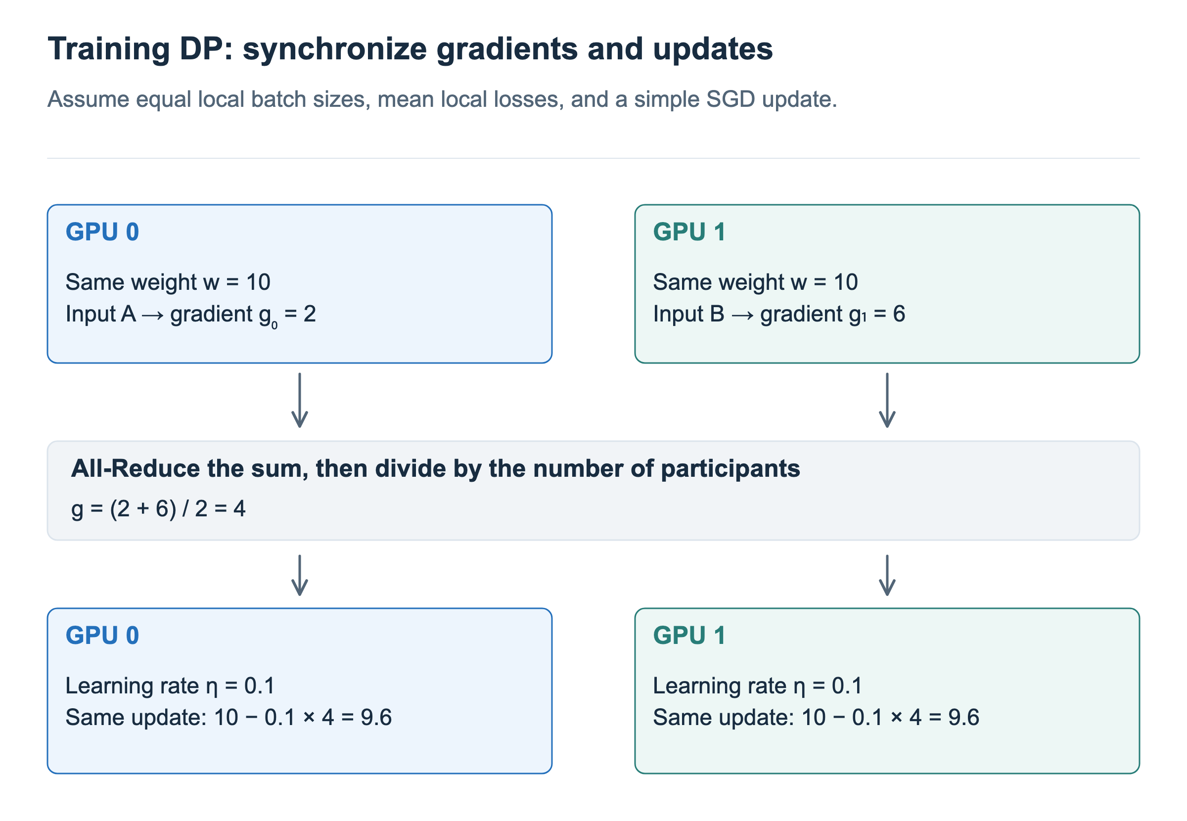
The figure starts with one weight at 10 and gradients 2 and 6 on the two GPUs. All-Reduce their sum and divide by two to obtain the same mean, 4, on both. With learning rate 0.1, a simple SGD update subtracts a scaled gradient, leaving both weights at 9.6. SGD is one method for updating weights.

PyTorch DDP synchronizes gradients between replicas. Implementations may group gradients or communicate those already available while computation continues. They need not wait for every computation and then perform exactly one communication as the simplified figure might suggest. Different local batch sizes or loss sum/mean conventions require checking the appropriate weighting and division.

Increasing Throughput by Dividing Inputs

DP distributes different inputs across replicas so they can complete more work in the same time. In inference, we can examine this benefit through the number of requests completed; in training, through the amount of data processed. Work processed per unit time is called throughput.

In inference, each replica handles different requests. The example below assumes four requests arrive together and each takes the same time to compute.

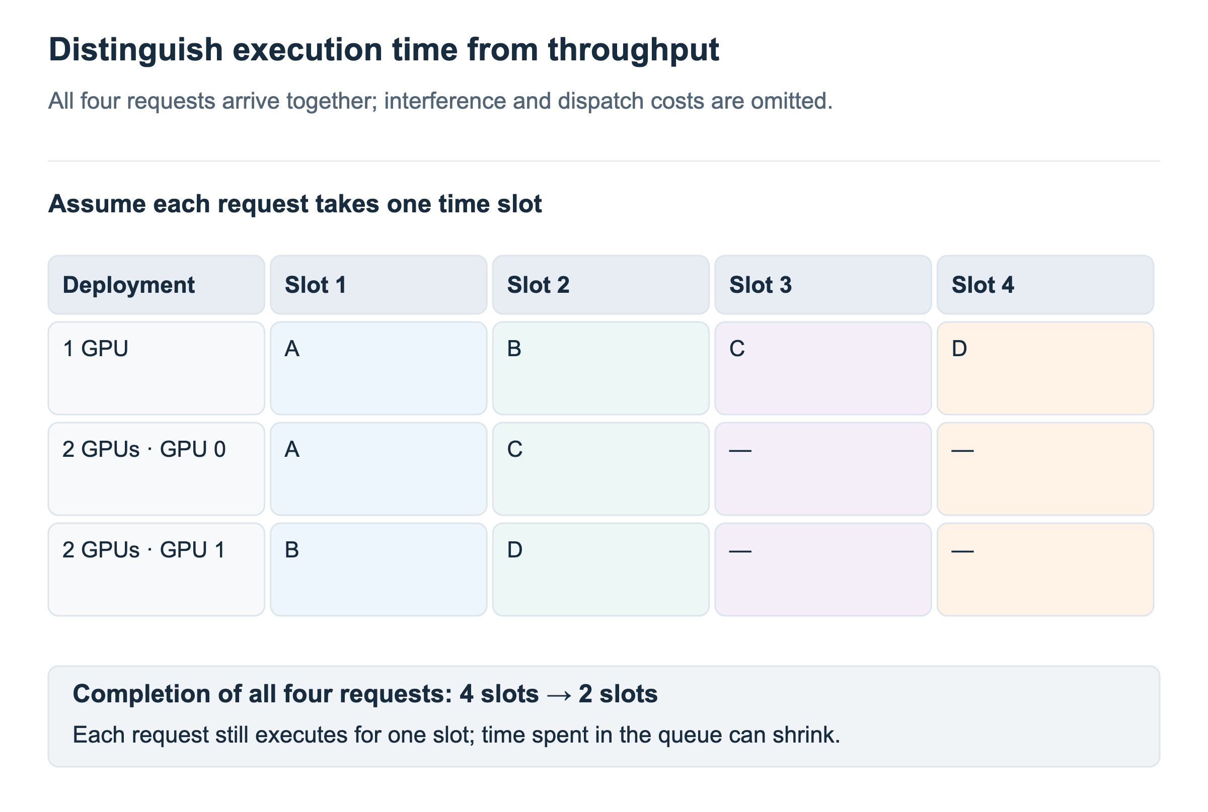
One GPU finishes four requests in four slots, while two GPUs finish them in two. All requests finish sooner, but each request still computes for one slot. The computation of an individual request has not been split. However, user-visible response time includes waiting before computation, so starting later requests earlier can also reduce their response time.

In training, replicas compute on different training data and combine their gradients to update the weights. Consider a workload where one GPU processes eight inputs before an update. If two GPUs each process eight inputs and combine their gradients, a single update can reflect sixteen inputs in total. This increases the total amount of data used at once while keeping each GPU’s share unchanged. In this example, the total number of inputs used for one update is the global batch size.

The global batch does not have to grow. We can keep eight inputs in total and have two GPUs compute four each. Here, the aim is to complete the same amount of computation sooner. Conversely, increasing the global batch also changes how much data each update uses, so higher data throughput does not imply a proportional reduction in the time needed to reach a target level of model performance.

In either case, throughput need not grow in proportion to GPU count. Too little input can leave GPUs idle, and smaller per-GPU batches may reduce compute efficiency. In training, waiting for the slowest participant’s gradients and synchronization costs also matter. Evaluate DP using request throughput and response time for inference, and data throughput together with global batch size for training.

A model too large to replicate, or a need to divide computation for the same input, calls for another placement. TP: Split One Operation Across GPUs examines the communication created by partitioning a matrix multiplication.