Prefill and Decode

In Inference and the KV Cache, we examined how storing K/V for past positions reduces repeated computation. Generation with a cache first processes the input context together, then processes one new input at a time while reading past KV. We call these two stages Prefill and Decode.

Both stages use the same model, but they compute different numbers of tokens at a time. In this article, we will examine how this difference affects computation and weight reuse. We will then use the Roofline model to compare their bottlenecks, and finally consider the cost of KV reads that remains even when processing multiple requests together.

The execution flow of Prefill and Decode

Prefill is the stage that first processes the supplied input context. If the input is p0 p1 p2 p3, the model processes all four positions together. It stores their K/V in the cache at each layer, then uses the prediction scores at the final input position, p3, to select the first output token, x0.

Decode is the stage that processes a new input token to select the next output token. When x0, selected during Prefill, enters as the next input, the model computes that position while attending to stored past K/V. It adds the newly computed K/V for x0 to the cache and uses the execution result to select the next output, x1. It then repeats the process, feeding in x1 to select x2.

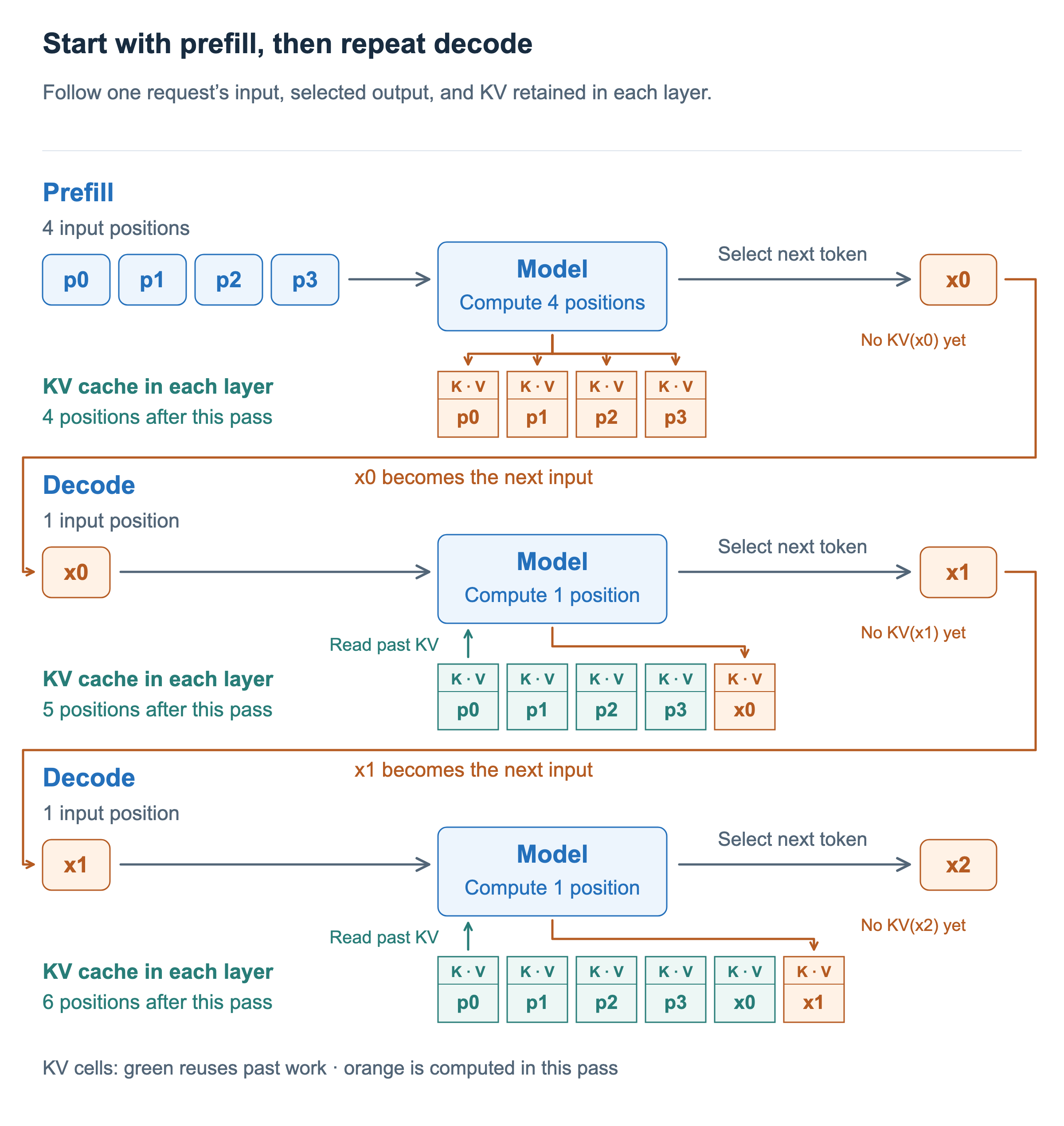
In Figure 1, Prefill processes four inputs together, while each Decode processes one input. The initially supplied inputs are already known, so they can be computed together. By contrast, a generated token is determined only after the preceding execution finishes. We cannot feed x0 into the next execution before selecting it.

The distinction between token selection and KV computation from the previous article still applies. Immediately after selecting x0, only KV for p0 through p3 exists. KV for x0 is created when x0 enters the next execution. Prefill’s result selects the first output token; repeated Decode executions select the outputs that follow.

Token count and attended context length

To understand the GPU’s work, we need to distinguish the number of tokens processed now from the context length that Attention accesses. Figure 2 shows a single request, using T for the current token count and L for the attended context length, including the current input.

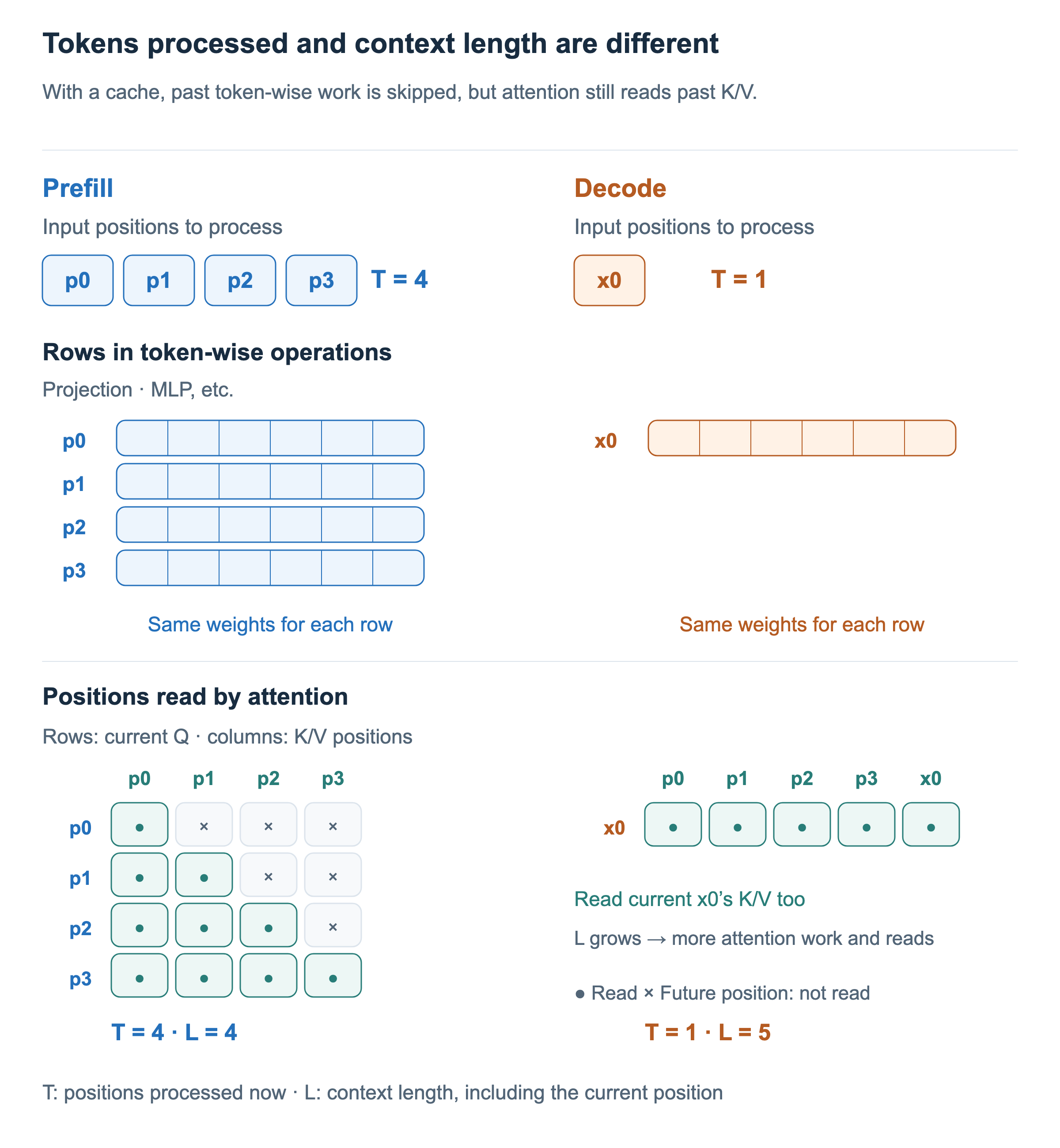
First, consider the token-wise operations at the top of the figure. The projections that create Q/K/V, the Attention output projection, and the matrix multiplications in the MLP apply the same weights to the vector at each token position. For a fixed model size, the computation in these linear operations is proportional to the number of tokens processed now. Prefill computes four rows, while the following Decode computes only one row for the new input, x0. It does not rerun projections or MLPs for past positions p0 through p3.

Attention, shown at the bottom, accesses a different range of positions. Rows represent the Q positions computed now, and columns represent the K/V positions they access. Prefill computes Q for all four positions together, but each position attends only to itself and earlier positions. The accessed cells therefore form a triangle. During Decode, one new Q attends to K/V for the four past positions and the current x0. Even with just one newly processed token, Attention uses five positions.

As generation continues and the context grows, ordinary Decode still receives one new input per request. A single request’s projection and MLP computation therefore stays roughly constant, while the KV accessed by Attention and the associated computation grow. This is why token count alone cannot explain the entire model’s computation. The Transformers cache explanation also shows how a new Q uses both past and current K/V.

Here, one token means one token per request, not per entire batch. If eight requests are grouped into one Decode batch, the execution processes eight new inputs in total. In the sections that follow, we will examine weight reuse in terms of this total number of tokens processed together in one execution.

Computing multiple tokens with the same weights

The model’s weights are the same during Prefill and Decode. Whether processing one token or several, the same linear layer needs the same weights. The difference is how many tokens we can compute with the weights we read.

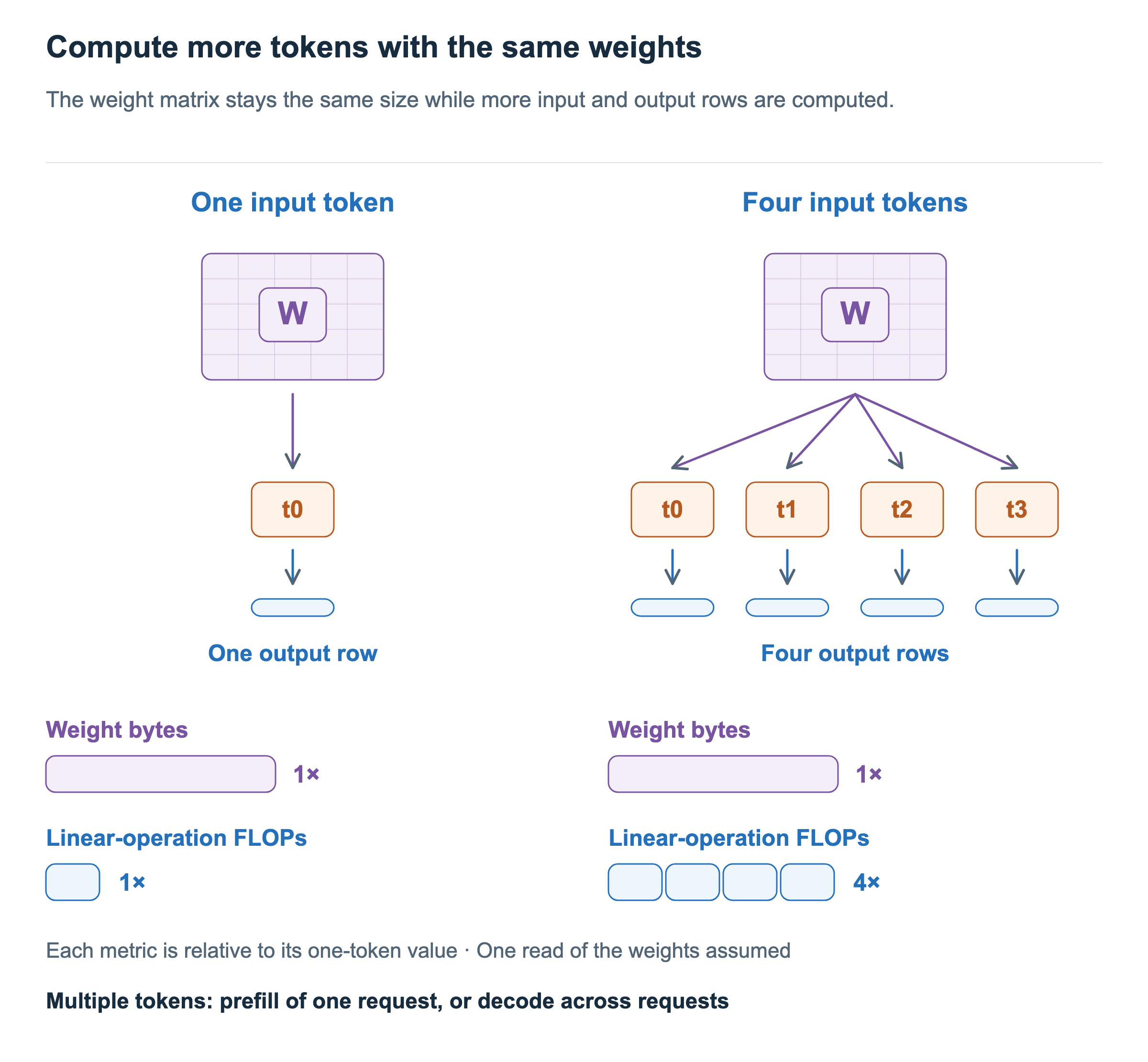
The left side of Figure 3 uses W to compute one input row. The right side computes four input rows with the same W. The amount of weight data stays the same, while the outputs to compute and the linear computation increase fourfold. Computing multiple inputs together lets us reuse weights fetched from memory across the rows. Both grouping one request’s Prefill tokens and grouping several requests’ Decode tokens create this opportunity.

For a linear operation with input and output dimensions d_in and d_out, respectively, the relationship is as follows. T is the number of tokens processed together in this execution.

X [T, d_in] × W [d_in, d_out] → Y [T, d_out]

Computation ≈ 2 × T × d_in × d_out FLOPs
Number of weight elements = d_in × d_out

Counting a multiplication and an addition as one FLOP each, computation grows in proportion to T. The size of W does not change. Thus, if weight reads account for a large share of data movement, processing more tokens together increases computation relative to the data moved. NVIDIA’s matrix multiplication performance guide also uses this ratio of computation to data movement to analyze bottlenecks.

The figure simplifies the comparison by assuming one read of the weights. In practice, inputs and outputs also move, and the kernel’s execution strategy and caching can cause the same weights to be read again. The relationship to focus on is the opportunity to reuse the same weights for more computation, rather than a fixed ratio of actual memory accesses.

Bottlenecks in Prefill and Decode

As we saw in Arithmetic Intensity and Roofline, arithmetic intensity is the ratio of computation to data movement. Here, we will consider the bytes read from and written to HBM, the GPU’s memory. Performing more computation for the same amount of data moved increases arithmetic intensity.

The Roofline model relates this ratio to the GPU’s memory bandwidth and compute performance. The horizontal axis is arithmetic intensity, and the vertical axis is computation performed per second. Execution must satisfy both the rate at which memory can supply data and the rate at which the compute units can perform calculations, so the lower of the two limits determines the throughput ceiling.

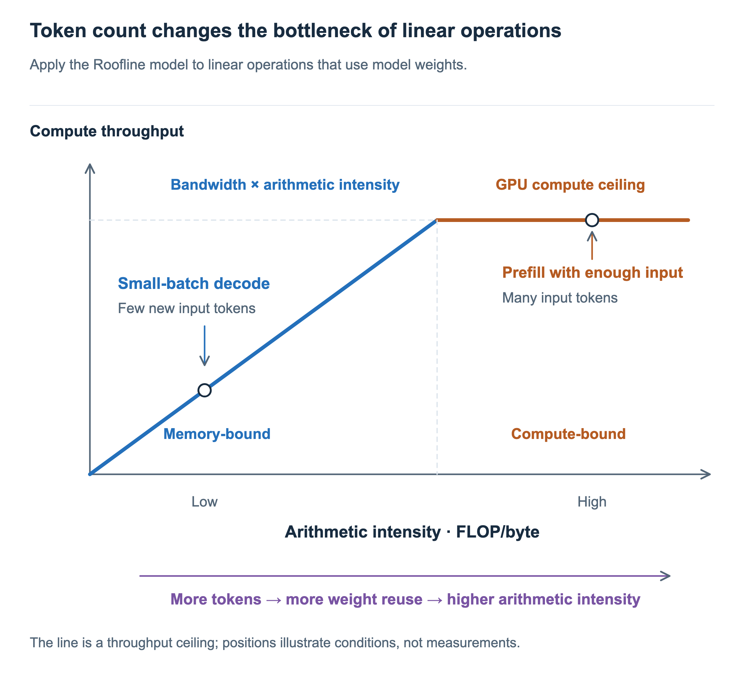
On the left side of Figure 4, there is little computation relative to the data moved. Even when the GPU has spare compute capacity, it cannot receive the required data quickly enough. We call this memory-bound. The memory limit here is the speed of data movement, rather than a shortage of storage space.

Small-batch Decode that must fetch a large model’s weights from HBM is likely to face this condition. With one request, there is only one new input to process, but its computation still needs the model’s weights. Reading many weights while performing little computation per value makes it difficult to fully use the GPU’s high compute performance.

On the right side of the figure, by contrast, computation is large relative to data movement, so the rate at which the compute units finish calculations determines the ceiling. We call this compute-bound. Prefill with a sufficiently long input processes many tokens together and reuses weights, making it easier for its linear operations to reach this condition. Even a single request can contain many tokens to process.

Decode also increases weight reuse in linear operations when it groups new inputs from multiple requests. The names Prefill and Decode therefore do not fix the bottleneck. What matters is the number of tokens processed together in one execution. Prefill with a short input and Decode with a large batch can occupy different positions from the examples shown in the figure.

This figure applies the Roofline model to linear operations that use weights. The lines and two markers illustrate performance ceilings and execution conditions; they are not measurements of a particular model. Actual throughput can fall below the ceiling depending on factors such as kernel execution efficiency, and the token count at which the bottleneck changes varies with the GPU, model, and data type.

Batching benefits and KV reads

So far, we have focused on weight reuse. Can we then solve the memory bottleneck by continuing to increase the Decode batch? In actual Decode, we also need to account for reading each request’s distinct KV cache, in addition to the weights.

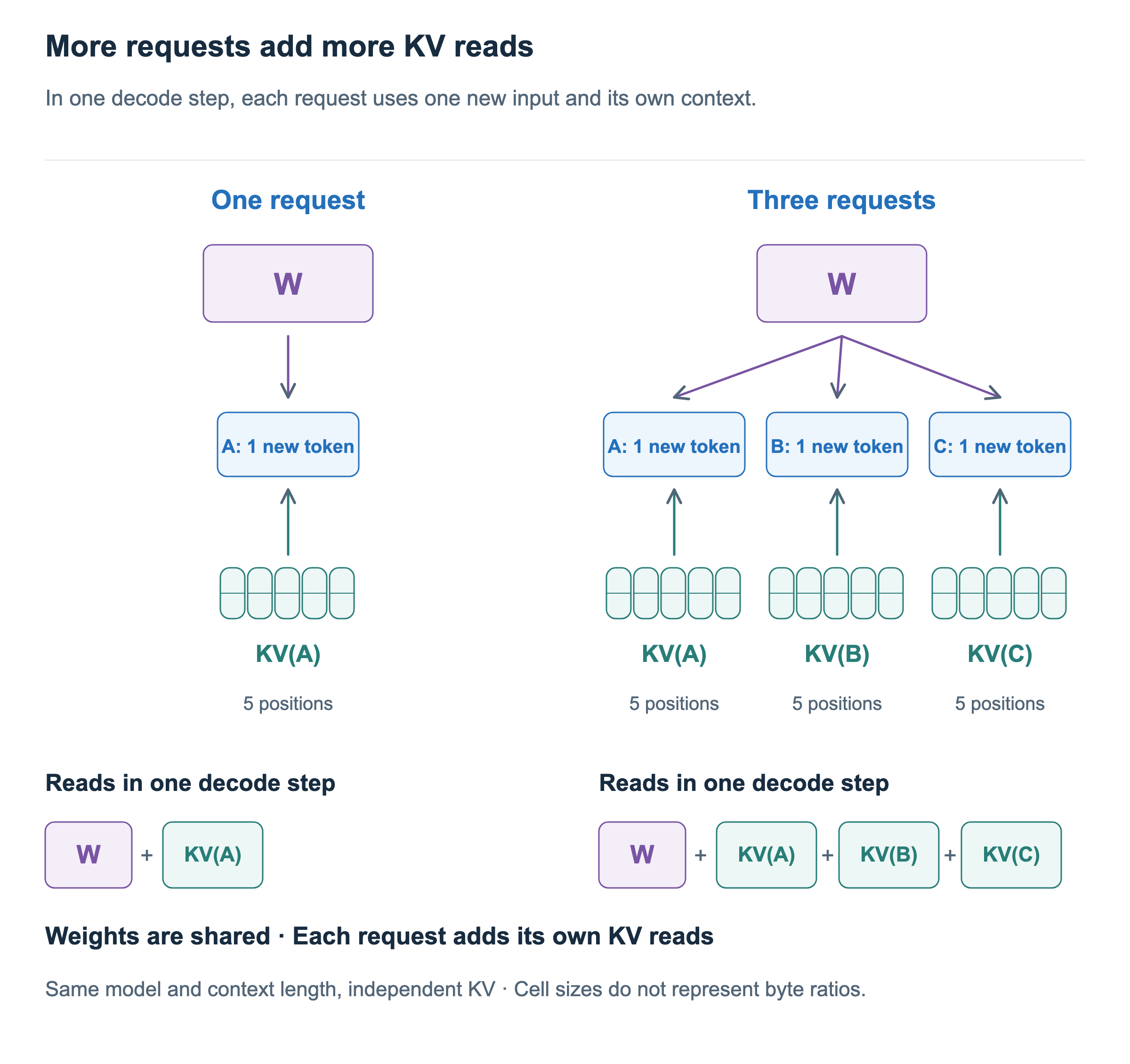
Figure 5 shows an example where each request attends to five positions, including its current input. Request A alone uses W and A’s KV. Processing B and C together with A reuses the same W for more token computation, but B’s and C’s KV must each be read as well. A longer context within one request also increases the KV that request reads. The JAX Scaling Book’s inference analysis likewise distinguishes the weight cost of linear operations from the KV cost of Attention.

Thus, batching can increase weight reuse, but it does not eliminate the cost of reading each request’s KV. In particular, as KV reads account for a larger share of the work, the benefit of increasing the batch becomes limited. This is why the preceding Roofline explanation of weight reuse cannot be extended unchanged to Decode as a whole.

Executing multiple requests together is an important way to improve Decode efficiency. In practice, however, requests have different arrival times and context lengths, and GPU resources are limited. Batching and Scheduling examines how to group these requests and decide what to include in the next execution.