Same Model, Different Workloads: Inference and Training

Having examined what a model computes and how a GPU executes that computation, we can now ask which inputs arrive and in what order the computation repeats. Even with the same Transformer, training on prepared data and answering user requests whose arrival times are unknown place different conditions on how we organize execution.

To describe these tasks, we must consider inputs, computation, retained state, repetition, and goals alongside the model’s name and size. Together, these make up a workload.

This article first examines how being able to prepare inputs in advance changes the execution plan. We will then compare token generation during inference with weight updates during training and look at the state each process retains. Finally, we will connect these ideas to the inference engine’s work, from receiving a new request to completing its response. Our comparison uses next-token training on prepared token sequences and inference that generates text for user requests with fixed model weights.

Training data and inference requests

The first difference in organizing a workload is when we know the inputs to process. If training data is ready, we can take the inputs and targets for each execution from that data. We can also plan which examples to group together and in what order to process them. The model does not have to generate an earlier answer before we can know the next training input.

In online inference, which receives user requests in real time, we cannot know in advance when future requests will arrive or what their content and length will be. Once a request arrives, its input is known, but new requests keep arriving while existing ones are in progress. The number of tokens a request will actually generate before ending may also be unknown when it starts.

For example, while the engine is answering request A, request B may arrive asking for a summary of a long document, followed by a short question C. The engine must continually consider both ongoing work and new requests to decide what to process first and how many requests to execute together. An important difference in online inference workloads is the shift from planning how to process prepared data to planning around requests that change during execution.

Inference can also process inputs collected in advance, such as a list of documents to summarize. In this offline setting, the upcoming inputs are known, but the computation that generates answers still differs from training computation that updates weights. Here, we focus on request management in online inference and compare it with training on prepared data.

Aspect	Inference: online generation	Training: prepared data
Input preparation	A request’s content becomes known when it arrives; later requests remain unknown	Prepare the inputs and targets for each execution from the data
Input	The prompt and outputs selected so far	A known token sequence containing the targets
Compute	Forward pass and next-token selection	Forward pass, loss, backward pass, and weight update
Repetition	Continue generation using the selected token	Continue training on the next data batch
Main state	Per-request token history and reusable KV	Activations needed for the backward pass, gradients, and optimizer state
Execution goals	Response time, throughput, and cost	Make progress with the available resources while maintaining training quality

The model defines the computation on given tensors. The engine prepares the required inputs and state and repeats that computation. We will examine training-engine design in detail when we turn to training.

Token generation and weight updates

Suppose we provide three tokens, p0 p1 p2, and ask the model to continue the sentence. The LM Head computes logits, the scores used to select the next token, from the representation at each input position. During generation, we use the logits at the final position, p2, to select a new token, x0. If generation continues, x0 becomes the input to the next execution, whose result selects x1.

During generation, the previously selected output becomes the input to the next execution. We cannot perform computation that takes x0 as input before selecting x0. This is why generation steps within a request remain sequential even when several requests execute together. Separately from the arrival times of new requests discussed above, a request’s answer also takes shape as generation proceeds.

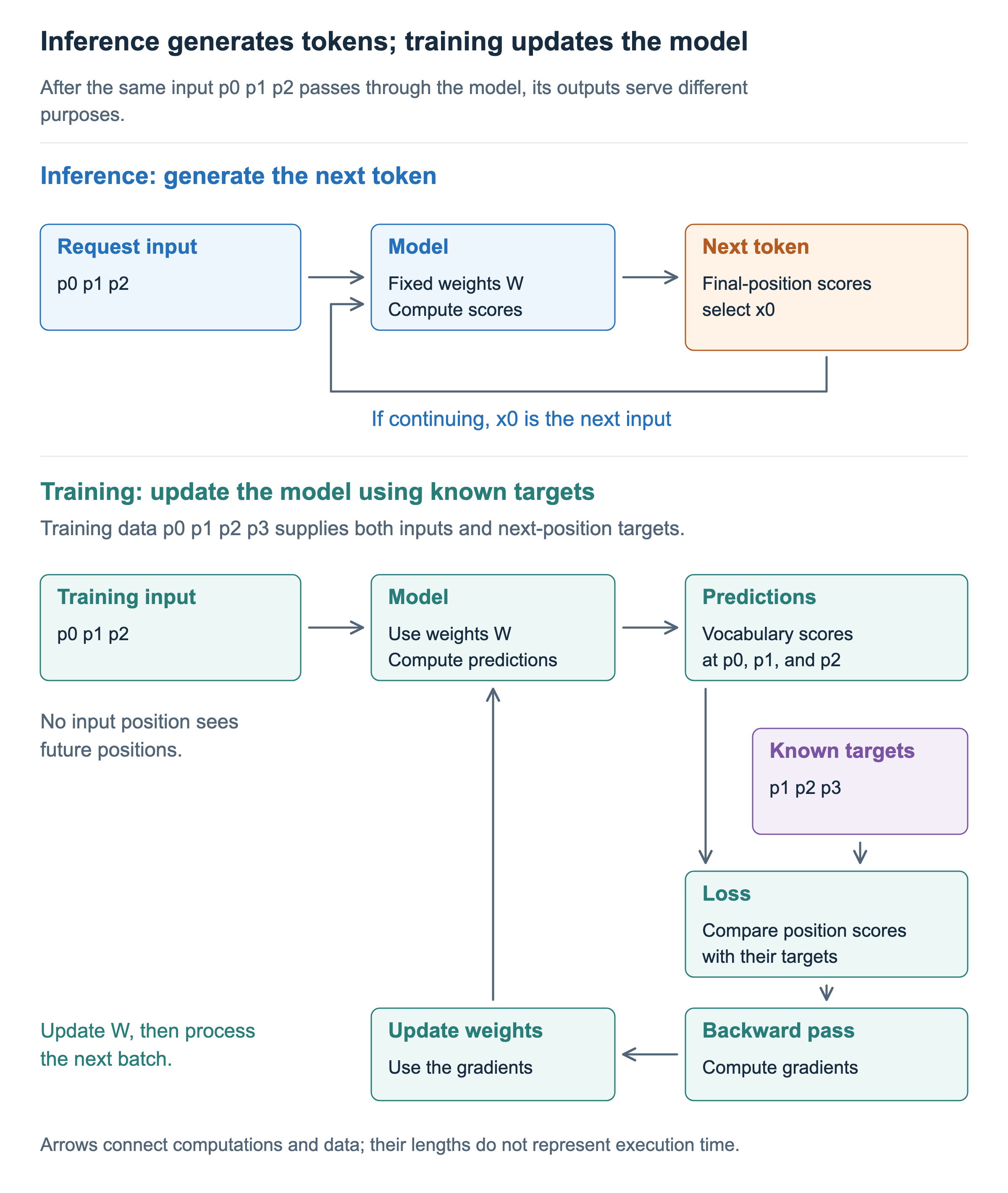
If the training data already contains p0 p1 p2 p3, the next-token targets for input p0 p1 p2 are p1 p2 p3. We can compute predictions at all three positions together and evaluate how much probability each prediction assigns to the target token. We obtain the next input and target from the data without waiting for the model to select a token at an earlier position. How next-token training works

Computing several positions together does not allow them to see the future. The causal mask prevents the position p0 from obtaining information from p1 or p2 through attention. The target p1 evaluates the prediction at p0, while the position p1 uses the context up to that position to predict the next token, p2. Using a known token sequence as input is distinct from the range of context each position may attend to.

Training measures how well the predictions match the targets through a loss. Rather than merely selecting one token and checking whether it matches the target, it evaluates the probability assigned to the target token. The backward pass obtains the gradients of the loss with respect to the weights, and the optimizer uses those gradients to update the weights. The next training batch uses the updated weights. Loss computation and weight updates

During inference, the weights remain fixed while the model repeats its forward pass and token selection. In the figure, the inference loop leads to the next input, while the training update leads back to the model weights.

State management in training and inference

Some information must remain available for the next task even after a model computation finishes. This state depends on the purpose of execution, as does the composition of GPU memory use. Both training and inference keep model weights in memory, but they retain different values in addition to those weights.

Training retains activations, intermediate values from the forward pass needed for the backward pass. It also needs gradients of the weights and optimizer state, such as accumulated statistics used to update the weights. Together with the weights, these values are major components of GPU memory use. Exactly what is stored, and how much, depends on the training method and optimizer: some activations may be recomputed when needed, or state may be placed in other memory.

Inference performs neither the backward pass nor weight updates, so it does not need gradients or optimizer state. Instead, the KV cache of requests being generated occupies GPU memory. A KV cache stores keys and values from earlier tokens for reuse when generating the next token. For now, the key point is that these values remain available as generation continues. The next article, Inference and the KV Cache, will explain what is stored and how it is reused.

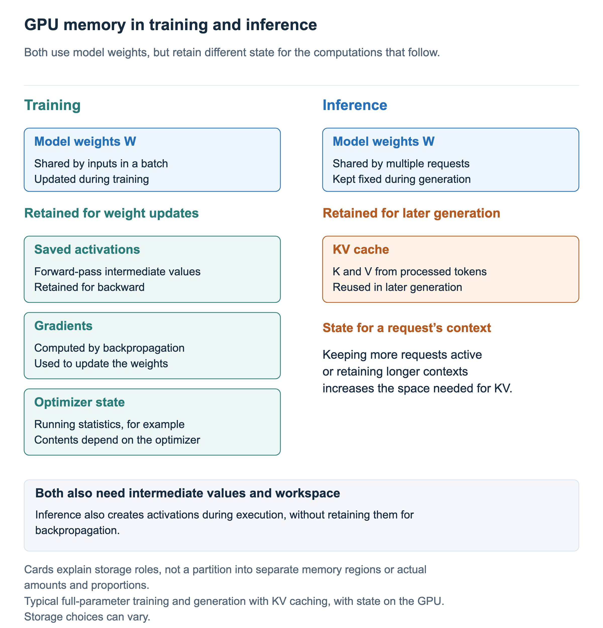
The figure compares major components; box sizes do not represent their actual shares of memory use. Inference also needs intermediate values and workspace for the current computation. The distinction to notice is why values are retained: training activations support the backward pass, while the KV cache supports subsequent generation.

Even when requests share the same model weights, the space needed for the KV cache grows as more requests run concurrently or each request retains a longer context. The KV cache is not always larger than the weights, but it is an important source of memory use that grows with requests. Knowing that the model weights fit on a GPU is therefore not enough to determine how many requests it can handle together.

Alongside this computational state, the engine manages each request’s input, selected output tokens, progress, and stopping conditions. Requests A and B can use the same model weights while retaining their own progress separately. This distinction will matter when we examine batching and scheduling.

How the inference engine handles requests

A sentence entered by a user does not immediately become a matrix multiplication on the GPU. The system must tokenize the text, prepare the request’s generation settings, and wait for an opportunity to execute. After execution, it must route results back to the corresponding requests, deliver output, and clean up resources belonging to completed requests. The inference engine connects these tasks to model execution. A real system may separate input processing, engine operations, and model execution into multiple components. vLLM architecture overview

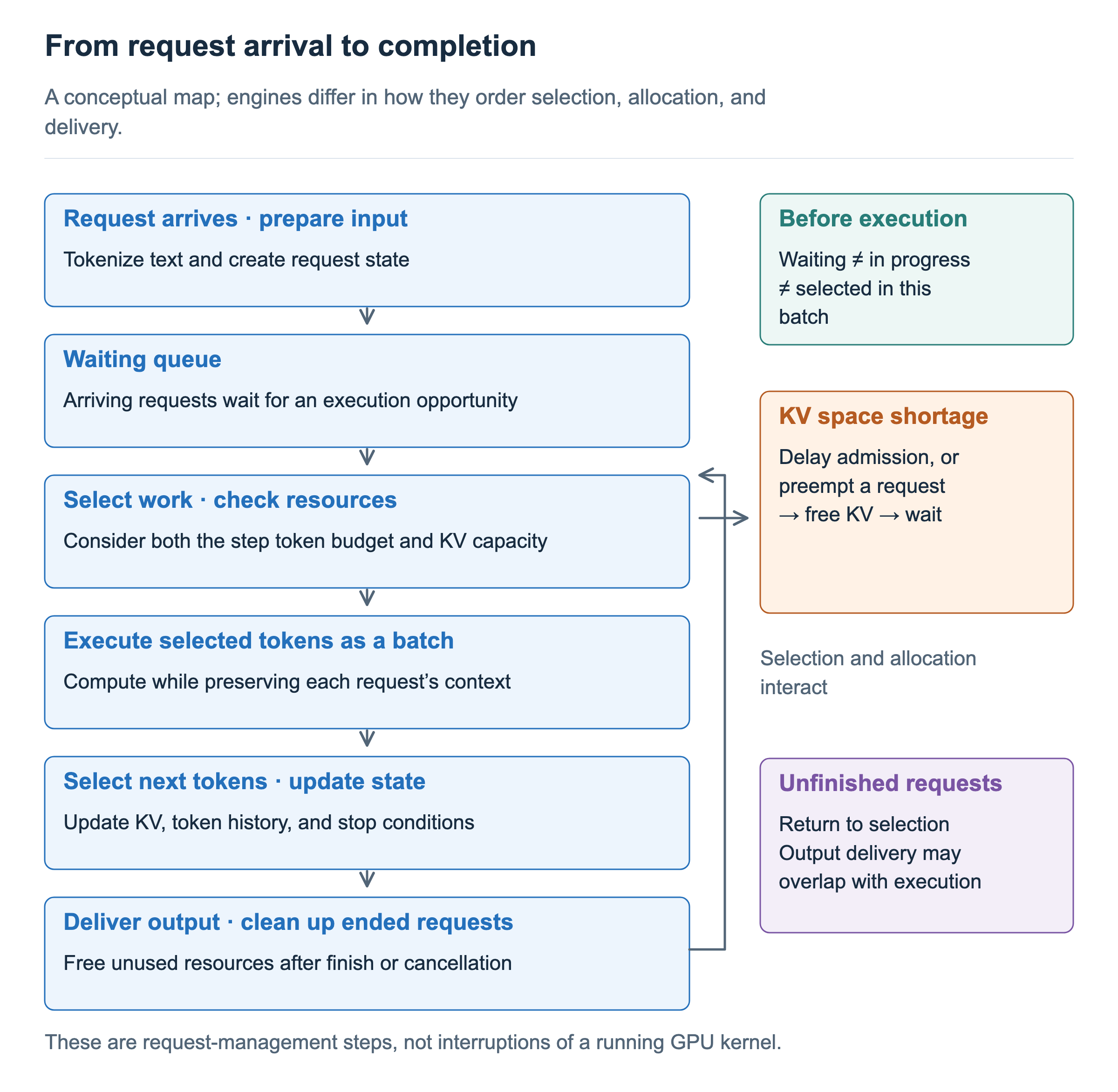
After input preparation, a new request enters a waiting queue. The engine selects work from ongoing and new requests for the next execution. A group of work from several requests executed together is a batch; choosing what to execute is scheduling.

Selection considers both the number of tokens to process in the current execution and the space available for KV storage. Adding more computation makes a step longer, while insufficient storage prevents the engine from retaining its results. Work selection and resource allocation must be coordinated.

After model execution, the engine incorporates newly computed KV and selected output tokens into request state. It delivers output to the user, and unfinished requests return to the set of candidates for the next step. Completed or canceled requests return resources that are no longer needed. Output delivery can overlap with the next computation, so the figure does not prescribe the exact function-call order of a particular engine.

Here, not every ongoing request participates in the same batch at every step. If the engine leaves some requests out to limit the current step’s token count, it can still retain their KV. When KV space is insufficient, the engine may instead need to delay new admissions or preempt an ongoing request and actually reclaim its KV storage. Removing a request from a batch and returning its storage are separate actions. We will examine preemption, reclamation, and resumption later; for now, remember that these are request-management decisions between model-execution steps.

Response time and throughput

Suppose request A needs a short answer, B is writing a long document, and C arrives while both are in progress. The engine must decide how to use the room left when A finishes first, how much more context B will retain, and when to start C. The actual output length may remain unknown until a request ends, so a single initial decision cannot easily determine the entire execution.

There is more than one goal. For conversational services, both a quick first response and steady subsequent output matter. When processing many documents in advance, completing the total workload within a time and cost budget may matter more. Running more requests together can improve server throughput without reducing each user’s waiting time by the same proportion. This is why we consider response-time constraints alongside throughput.

Training also aims to make progress with the same resources while maintaining training quality. We will not reduce this distinction to “training is always compute-bound and inference is always memory-bound.” Even within generation, processing the input context has a different computational shape from extending the output one token at a time. A later article on Prefill and Decode will examine that distinction.

Although SFT is generally included in post-training, our series follows a teaching sequence that places pretraining and SFT in the training stage, followed by RL-based post-training. RL-based processes connect the two execution patterns, for example by using generated results for training.

Having examined how the inference engine handles requests, we will next look more closely at how a single request generates tokens. In Inference and the KV Cache, we will follow what is newly computed and which earlier computations are reused when calculating the next token.