Inference and the KV Cache

In Same Model, Different Workloads: Inference and Training, we saw how inference generates the next token while keeping the model weights fixed. The selected token becomes input again, and the model predicts the token that follows it. If we compute the entire context from scratch each time, computation over the prefix we have already processed repeats as well.

This article follows a single request generating one token at a time. We will first identify the repeated computation, then connect it to storing past K/V to reduce that work. Finally, we will distinguish tokens selected as output from positions whose KV has been computed.

Generating tokens one at a time

Let the input tokens be p0 p1 p2. Here, p denotes the initial input, and x denotes output tokens selected during generation. These are illustrative symbols; one token does not necessarily correspond to one word.

Passing the input through the model computes a representation at each position. The LM Head uses this representation to produce logits, prediction scores for tokens in the vocabulary. To generate the next token, we use the scores at the final input position. Here, scores at p2 select the first output, x0. We can choose the highest-scoring token or draw one from a probability distribution derived from the scores.

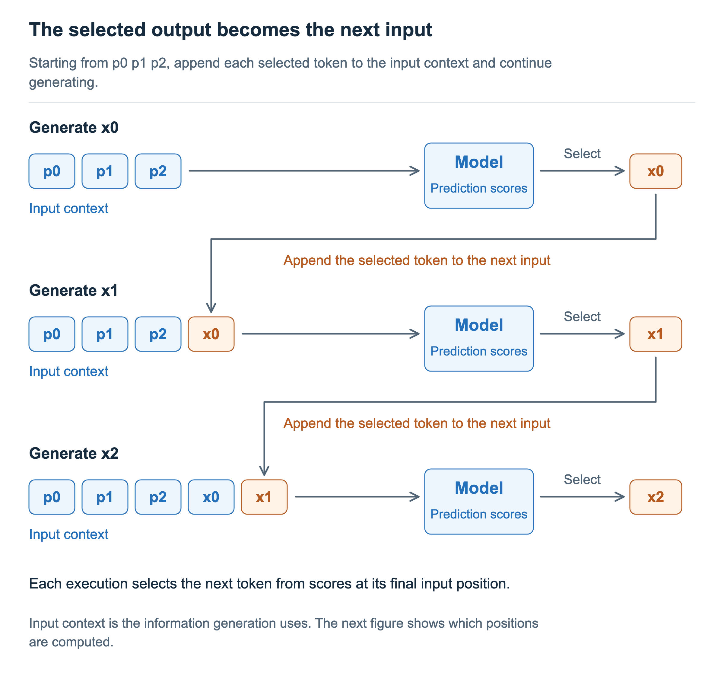
After selecting x0, the context for the next prediction becomes p0 p1 p2 x0. We use this context to select x1, then append x1 to select x2. The arrows returning from the output on the right to the input in the next row show this repetition. The next input token is determined only after the current token has been selected.

Input context here means all the information the next prediction attends to. Whether using that information requires recomputing every position each time is a separate question. Let us examine how to reduce computation while keeping the same generation process.

Repeated computation without a cache

The simplest implementation feeds the entire current context into the model each time. It computes p0 p1 p2 first, then p0 p1 p2 x0, and then p0 p1 p2 x0 x1. Every time one new token is added, the prefix also passes through the model again.

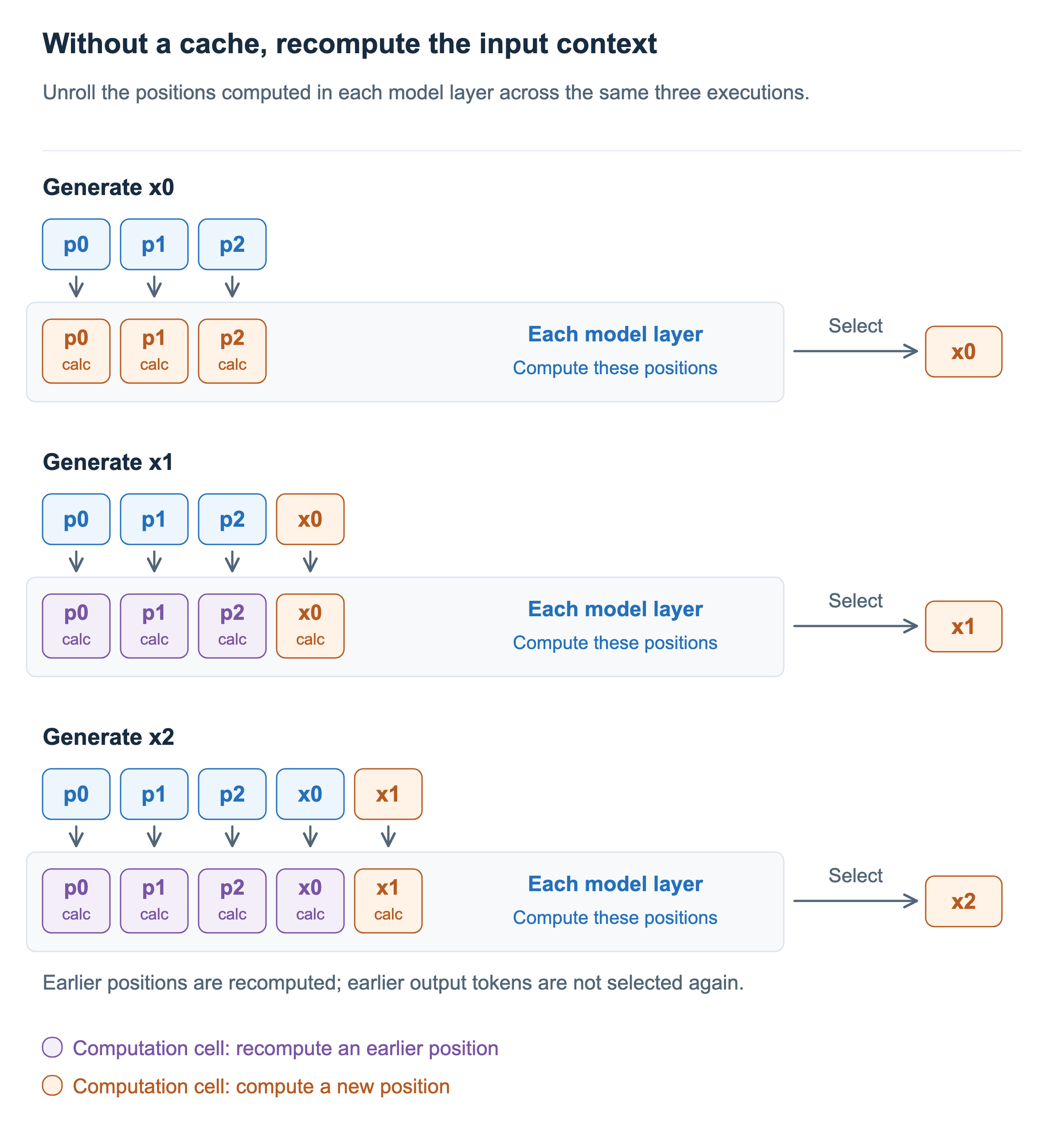
Orange computation cells mark positions being processed for the first time, while purple computation cells mark positions that were already processed and are now being recomputed. The execution that selects x1 computes the new input x0 and also repeats the computation for p0 p1 p2. At each layer, it recreates K/V at past positions and runs attention and MLPs again.

When selecting x2, it recomputes not only p0 p1 p2 but also the previously processed x0. This does not change output tokens that have already been selected. The token history stays the same while computation results for those input positions are recreated.

As generation continues, each position is computed more times. If results at past positions remain valid, we can retain the values needed by the next execution and reduce this repetition.

Reusing past computation with the KV cache

The KV cache stores keys and values computed at earlier input positions for reuse in later executions. This differs from storing token IDs themselves. Even the same token can have different K/V when its preceding context or position differs, so here we reuse K/V from positions already processed within the same request.

Causal attention explains why we can keep using past computation. A position attends only to itself and earlier positions. For example, p1 attends to p0 p1, but not to x0, which is added later. In ordinary inference with the same inputs, positions, and weights, adding x0 therefore does not change the computation result at the earlier position p1.

This property holds at each layer. Attention at past positions cannot see future positions, and token-wise operations such as normalization and MLPs do not mix in future positions either. By retaining K/V already computed at each layer, we can process a new position without rerunning computation at past positions. Transformers explanation of KV reuse

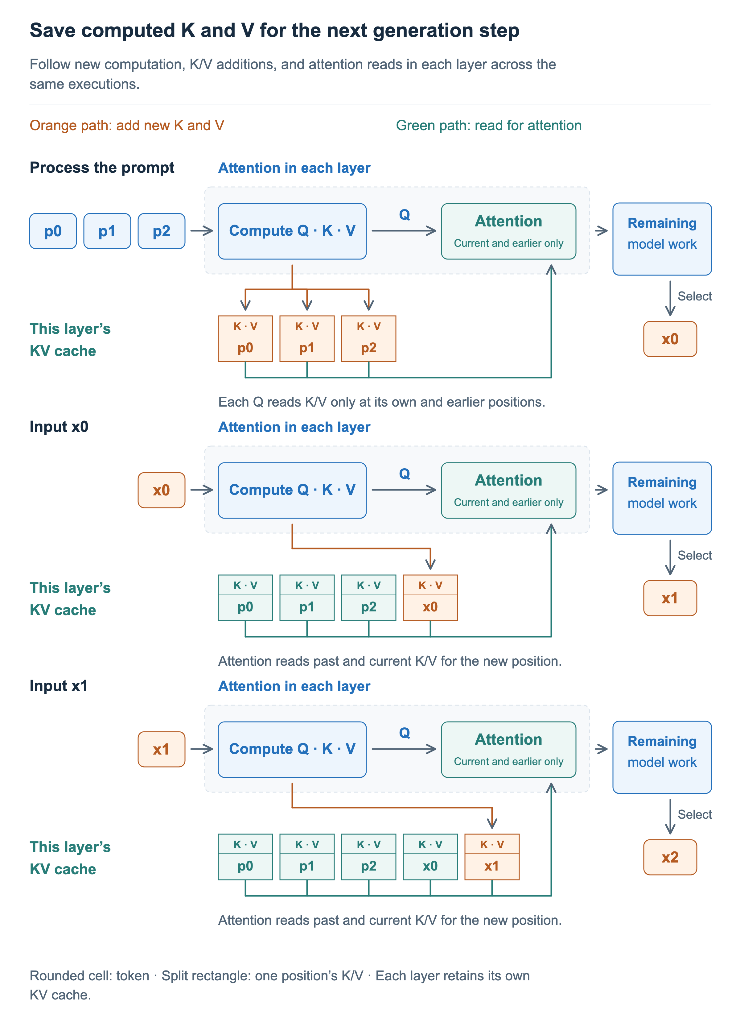
The figure expands the attention part of each model layer. Rounded cells are input and output tokens; split rectangles labeled with K/V and a position are stored computation results. Orange paths add new K/V to the cache, while green paths show attention reading K/V.

First, we process p0 p1 p2 and store their K/V at each layer. When x0 then becomes input, we compute new Q/K/V for that position, and Q(x0) attends to K/V for both the past positions p0 p1 p2 and the current position x0. The newly computed K/V for x0 remains in the cache. Processing x1 next adds its K/V in the same way.

We do not need to retain Q at past positions. Computing attention for x0 requires Q(x0) and the K/V of the positions it attends to. It does not reuse Q from the already processed positions p0 p1 p2. At each layer, the relationship is:

Current attention = Attention(new Q, [past K, new K], [past V, new V])

The brackets mean that past and current K/V are accessed together. With a cache, the new input position passes through each layer’s computation, while repeated computation at past positions can be skipped. Attention at the new position still needs to read past K/V. The context information has not disappeared: we use stored values instead of computing them again.

The boundary between token selection and KV computation

Notice that input and output in the figure are offset by one token. Immediately after processing the initial input p0 p1 p2 and selecting x0, KV is ready for the three input positions. But the just-selected token x0 does not yet have its own KV. The model computed representations for the positions it received as input; x0 was chosen as the next token using that computation’s result.

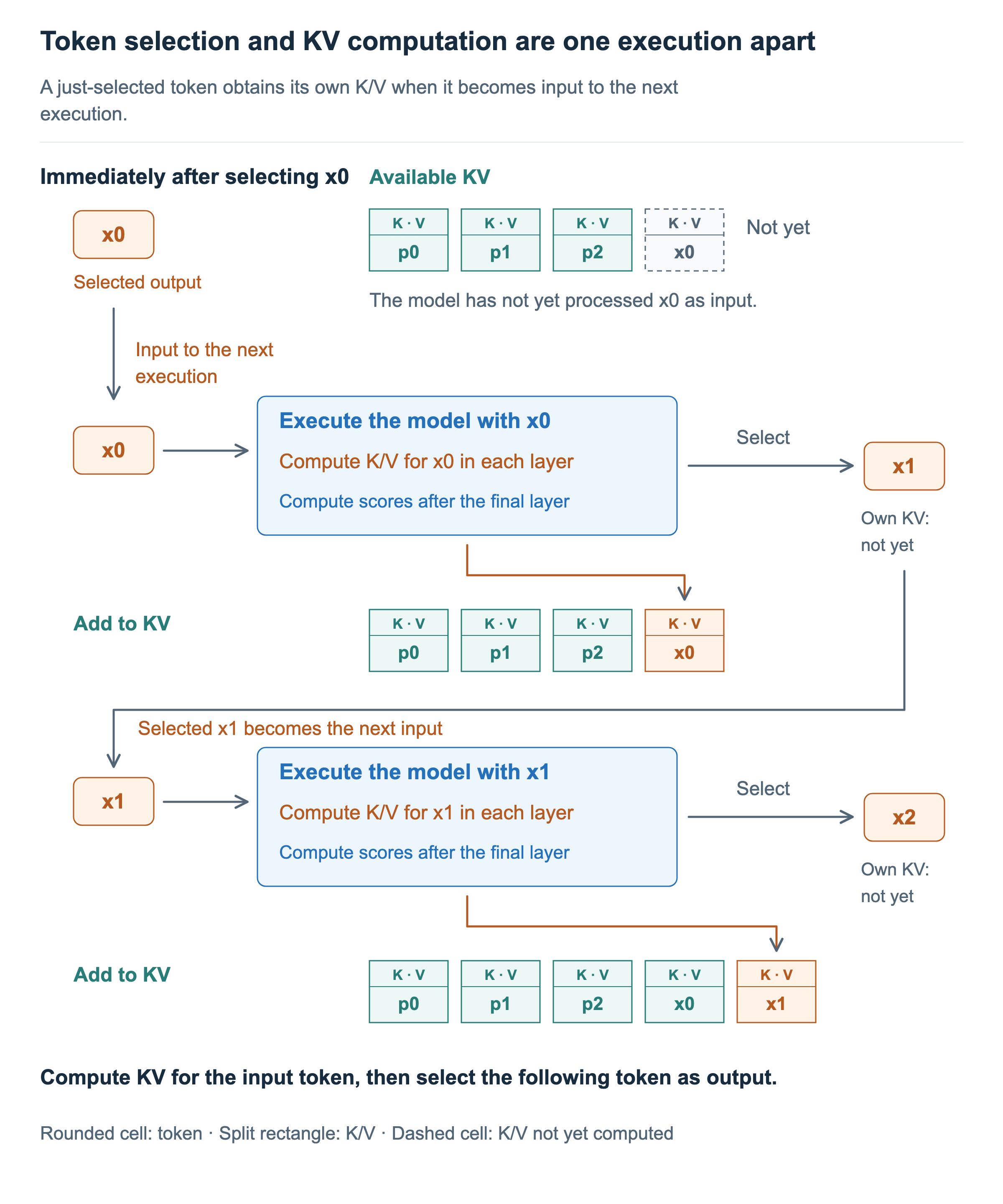
The next execution takes x0 as input. At each layer, the model computes its K/V and builds its representation while attending to past K/V. Scores obtained through the final layer and LM Head select x1. The cache is now ready through p0 p1 p2 x0, but the newly selected x1 does not yet have its own KV.

When x1 becomes the next input, its KV is created and x2 is selected. In the figure, an output token connects to the input of the next execution, while K/V computed inside the model is added to the cache. Selecting a token and computing its K/V happen in different executions. At the same instant, the token history can include x1 while KV is ready only through the preceding token, x0.

Distinguishing this boundary makes clear what the next execution needs to compute. It reuses past positions whose KV is already available and computes the just-selected, still-unprocessed token as new input. Repeating this process extends both the output and the KV cache.

Initially, we processed the given input context together. Later, we processed one new input while reading past KV. In the next article, we will name these two executions prefill and decode and examine how the number of tokens computed together and the length of the attended context affect computation and memory reads.