Shared Concepts · Hardware · 2026-09-18
SP: Partition Activations Alongside TP
Reduce activation duplication between TP regions, and alternate between token and feature partitioning to compute a Transformer layer.
In tensor parallelism (TP), multiple GPUs split the computation for the same input. They partition attention heads or intermediate FFN features, then combine the final partial sums. But splitting these large matrix multiplications does not partition every value and operation in a layer. All-Reduce gives each GPU the same complete result, and the following normalization processes that same input redundantly.
Intermediate values produced during model computation are called activations. This article first examines which activations remain replicated between TP regions. We then see why normalization and residual connections can be partitioned by token, and follow the layout changes when entering and leaving TP. Finally, we connect these boundaries across an entire Transformer layer.
Here, sequence parallelism (SP) refers to the method proposed in Megatron. It partitions tokens from the same input, rather than assigning different requests or training samples to GPUs as DP does. The figures show a forward pass on two GPUs.
Activation duplication between TP regions
Start with a layer that uses TP alone. Rows in the small matrices represent tokens, and columns represent features. Inside attention, each GPU holds values for its assigned heads. Inside the FFN, it holds its assigned intermediate features. These are regions where the GPUs compute different parts.
However, the outputs of attention’s Output Projection and the FFN’s final Linear are still partial sums. In the basic TP configuration we examined earlier, All-Reduce adds these contributions and gives both GPUs the full result.
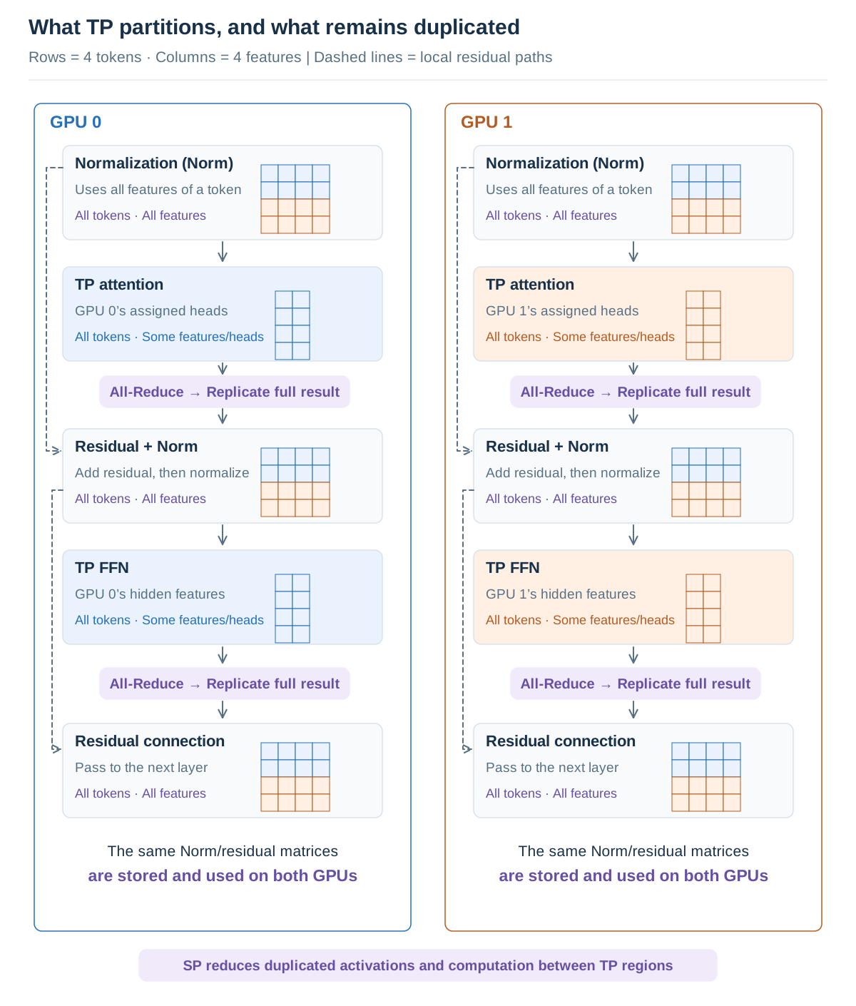
The matrices in the normalization and residual regions are identical on both GPUs. With four tokens and four features per token, each GPU stores the same 4×4 array. Normalization also processes the same four tokens twice.
SP changes the layout in these regions so that each GPU holds and processes activations for only some tokens. It keeps TP’s partitioning of the large attention and FFN matrix multiplications while reducing the replication and redundant computation between them.
Normalize and add residuals by token
Suppose GPU 0 holds tokens t0 and t1, and GPU 1 holds t2 and t3. Each GPU’s activations shrink from the full 4×4 array to a 2×4 shard. The important point is that all four features of a token stay together. We split whole token vectors between GPUs, rather than cutting each token’s features in half.
This layout keeps the values needed for normalization on one GPU. RMSNorm uses a token’s features to adjust its scale. It does not need other tokens’ features, so GPU 0 can normalize t0 and t1 without receiving t2 and t3.
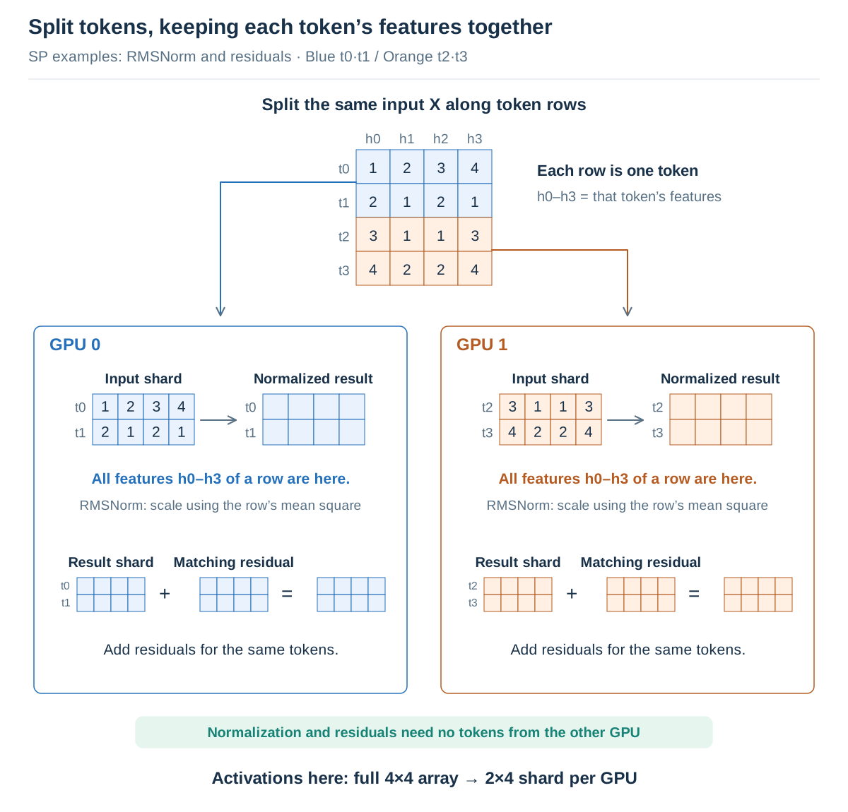
A residual connection also adds corresponding features of the same token. GPU 0 can finish the addition if it holds both the computed result and the residual for t0 and t1. The input retained as a residual must therefore use the same token layout as the result. The addition at the bottom of the figure illustrates this condition.
This does not mean that FFNs use TP because they cannot operate independently by token. FFNs also process each token independently. In this configuration, however, their large weight matrices and computation are partitioned with TP. SP preserves that setup while partitioning activations in the normalization and residual regions. The partitioning axis depends not only on dependencies between tokens, but also on where weights reside and what input the next operation needs.
Change layouts between SP and TP
After normalization, we need to compute TP’s first Linear. Each GPU holds different columns of the weight matrix. GPU 0 must compute the leading output features for every token, and GPU 1 the remaining output features for every token. Both therefore need the input for all tokens.
We gather the token shards with All-Gather. The t0–t1 and t2–t3 shards from the SP region combine into the same input X on both GPUs. We can then connect TP’s column and row partitions as before. Use Next in the following figure to follow a small FFN computation.
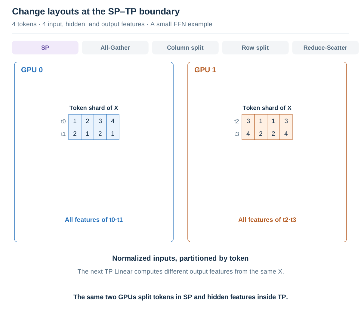
SP token shardsView the completed figure
Use Next to follow the computation. Click the figure to enlarge it.
The first Linear multiplies X by column shards of weight matrix U. GPU 0 computes intermediate features f0 and f1, while GPU 1 computes f2 and f3. Both process every token, but take responsibility for different features. Each value is a complete output feature, so an elementwise activation can be applied immediately. The figure uses a small ReLU example in which positive values remain unchanged; actual models may use other activations.
The second Linear multiplies this feature shard by the corresponding rows of weight matrix V. No communication is needed to gather the intermediate values, but the resulting P0 and P1 are partial sums for the same output positions. For example, t0’s first output feature is completed by adding GPU 0’s 4 and GPU 1’s 5 to obtain 9.
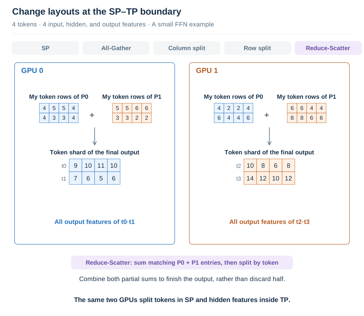
If the next region also uses SP, every GPU does not need the entire completed output. Reduce-Scatter adds the partial sums and distributes the result by token. In the final step, GPU 0 retains the complete outputs for t0 and t1, and GPU 1 retains those for t2 and t3. Each GPU does not simply cut its own partial result in half: it incorporates the other GPU’s contribution to complete the values for its tokens.
The GPU group does not change during this process. The same two GPUs partition tokens in SP regions and intermediate features inside TP. All-Gather and Reduce-Scatter form the boundaries connecting these layouts.
Connect SP and TP across a layer
We have followed the FFN, but the same structure appears around attention. The figure below shows a Pre-Norm layer, which applies normalization first. Dashed lines show residuals retained on the same GPU and added later; purple denotes collectives involving both GPUs.
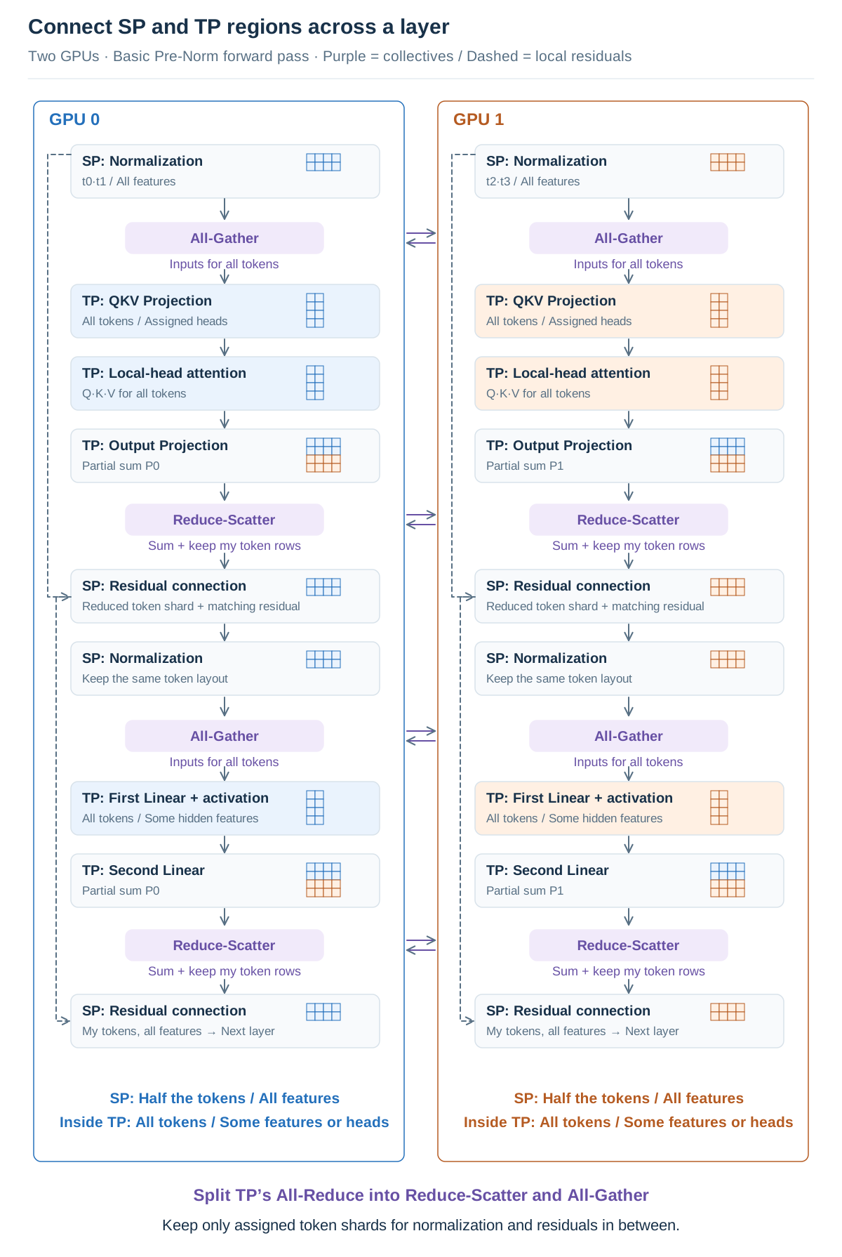
Each GPU first normalizes its own tokens, then All-Gather combines the inputs. TP’s QKV Projection uses that input to produce Q, K, and V for the assigned heads. At this point, all tokens for an assigned head are on one GPU, so computing that head’s attention does not require fetching additional tokens from another GPU.
Continuing the per-head computation through Output Projection produces partial sums on each GPU. Reduce-Scatter combines them and partitions the result by token. The SP region then adds the residual and applies normalization again. The FFN follows All-Gather → TP computation → Reduce-Scatter, and the final residual connection passes each GPU’s token activations to the next layer.
This structure does not simply add communication on top of TP’s existing All-Reduce. As we saw in collective communication, the result of All-Reduce can be obtained by Reduce-Scatter followed by All-Gather. SP places regions that only need the reduced shards between those two operations, gathering the data when the next TP computation requires the full input. This layout works because normalization and residual connections can operate on the shards in between.
Activation savings and total execution cost
SP directly reduces the activations each GPU stores and processes in the relevant regions. During training, activations are often retained for backpropagation, so these savings can become more important as sequences grow longer.
This does not halve total GPU memory usage. TP regions need gathered inputs, and communication buffers and other intermediate values also exist. SP itself does not change the weight placement either. The size of a particular array in a figure must therefore be distinguished from peak memory usage during actual execution.
Communication does not disappear. Even when All-Reduce and the combination of Reduce-Scatter and All-Gather correspond in transferred volume for the same data size, their execution time can differ with invocation timing, buffers, and overlap with computation. Inference also differs from training in the number of tokens processed at once and the state retained, so training benefits do not transfer unchanged.
In this configuration, we gathered the full token input before TP attention. What if each GPU were to handle only some tokens even in attention? We would need to handle the dependency between local Q and K/V on another GPU. The next article on context parallelism (CP) examines how to preserve this connection while partitioning a long context.